Operationalize ML In Your Data Pipelines with Snowflake Cortex

Overview

This entry-level Hands-On Lab exercise is designed to help you master the basics of Coalesce. In this lab, you’ll explore the Coalesce interface, learn how to easily transform and model your data with our core capabilities, understand how to deploy and refresh version-controlled data pipelines, and build a ML Forecast node that forecasts sales values for a fiction food truck company.

What You’ll Need

A Snowflake trial account
A Coalesce trial account created via Snowflake Partner Connect
Basic knowledge of SQL, database concepts, and objects
The Google Chrome browser

What You’ll Build

A Directed Acyclic Graph (DAG) representing a basic star schema in Snowflake

What You’ll Learn

How to navigate the Coalesce interface
How to add data sources to your graph
How to prepare your data for transformations with Stage nodes
How to join tables
How to apply transformations to individual and multiple columns at once
How to build out Dimension and Fact nodes
How to make changes to your data and propagate changes across pipelines
How to configure and build an ML Forecast node

By completing the steps we’ve outlined in this guide, you’ll have mastered the basics of Coalesce and can venture into our more advanced features.

About Coalesce

Coalesce is the first cloud-native, visual data transformation platform built for Snowflake. Coalesce enables data teams to develop and manage data pipelines in a sustainable way at enterprise scale and collaboratively transform data without the traditional headaches of manual, code-only approaches.

What Can You Do With Coalesce?

With Coalesce, you can:

Develop data pipelines and transform data as efficiently as possible by coding as you like and automating the rest, with the help of an easy-to-learn visual interface
Work more productively with customizable templates for frequently used transformations, auto-generated and standardized SQL, and full support for Snowflake functionality
Analyze the impact of changes to pipelines with built-in data lineage down to the column level
Build the foundation for predictable DataOps through automated CI/CD workflows and full git integration
Ensure consistent data standards and governance across pipelines, with data never leaving your Snowflake instance

How Is Coalesce Different?

Coalesce’s unique architecture is built on the concept of column-aware metadata, meaning that the platform collects, manages, and uses column- and table-level information to help users design and deploy data warehouses more effectively. This architectural difference gives data teams the best that legacy ETL and code-first solutions have to offer in terms of flexibility, scalability, and efficiency.

Data teams can define data warehouses with column-level understanding, standardize transformations with data patterns (templates) and model data at the column level.

Coalesce also uses column metadata to track past, current, and desired deployment states of data warehouses over time. This provides unparalleled visibility and control of change management workflows, allowing data teams to build and review plans before deploying changes to data warehouses.

Core Concepts in Coalesce

Coalesce currently only supports Snowflake as its target database, As you will be using a trial Coalesce account created via Partner Connect, your basic database settings will be configured automatically and you can instantly build code.

Organization

A Coalesce organization is a single instance of the UI, set up specifically for a single prospect or customer. It is set up by a Coalesce administrator and is accessed via a username and password. By default, an organization will contain a single Project and a single user with administrative rights to create further users.

Projects

Projects provide a way of completely segregating elements of a build, including the source and target locations of data, the individual pipelines and ultimately the git repository where the code is committed. Therefore teams of users can work completely independently from other teams who are working in a different Coalesce Project.

Each Project requires access to a git repository and Snowflake account to be fully functional. A Project will default to containing a single Workspace, but will ultimately contain several when code is branched.

Workspaces VS Environments

A Coalesce Workspace is an area where data pipelines are developed that point to a single git branch and a development set of Snowflake schemas. One or more users can access a single Workspace. Typically there are several Workspaces within a Project, each with a specific purpose (such as building different features). Workspaces can be duplicated (branched) or merged together.

A Coalesce Environment is a target area where code and job definitions are deployed to. Examples of an environment would include QA, PreProd, and Production.

It isn’t possible to directly develop code in an Environment, only deploy to there from a particular Workspace (branch). Job definitions in environments can only be run via the CLI or API (not the UI). Environments are shared across an entire project, therefore the definitions are accessible from all workspaces. Environments should always point to different target schemas (and ideally different databases), than any Workspaces.

Lab Use Case

As the lead Data & Analytics manager for TastyBytes Food Trucks, you're responsible for building and managing data pipelines that deliver insights to the rest of the company. There customer-related questions that the business needs to answer that will help with inventory planning and marketing. Included in this, is building a machine learning forecast that will allow management to determine sales volume for each item on the menu.

In order to help your extended team answer these questions, you’ll need to build a customer data pipeline first.

Before You Start

To complete this lab, please create free trial accounts with Snowflake and Coalesce by following the steps below. You have the option of setting up Git-based version control for your lab, but this is not required to perform the following exercises. Please note that none of your work will be committed to a repository unless you set Git up before developing.

We recommend using Google Chrome as your browser for the best experience.

Note: Not following these steps will cause delays and reduce your time spent in the Coalesce environment.

Step 1: Create a Snowflake Trial Account

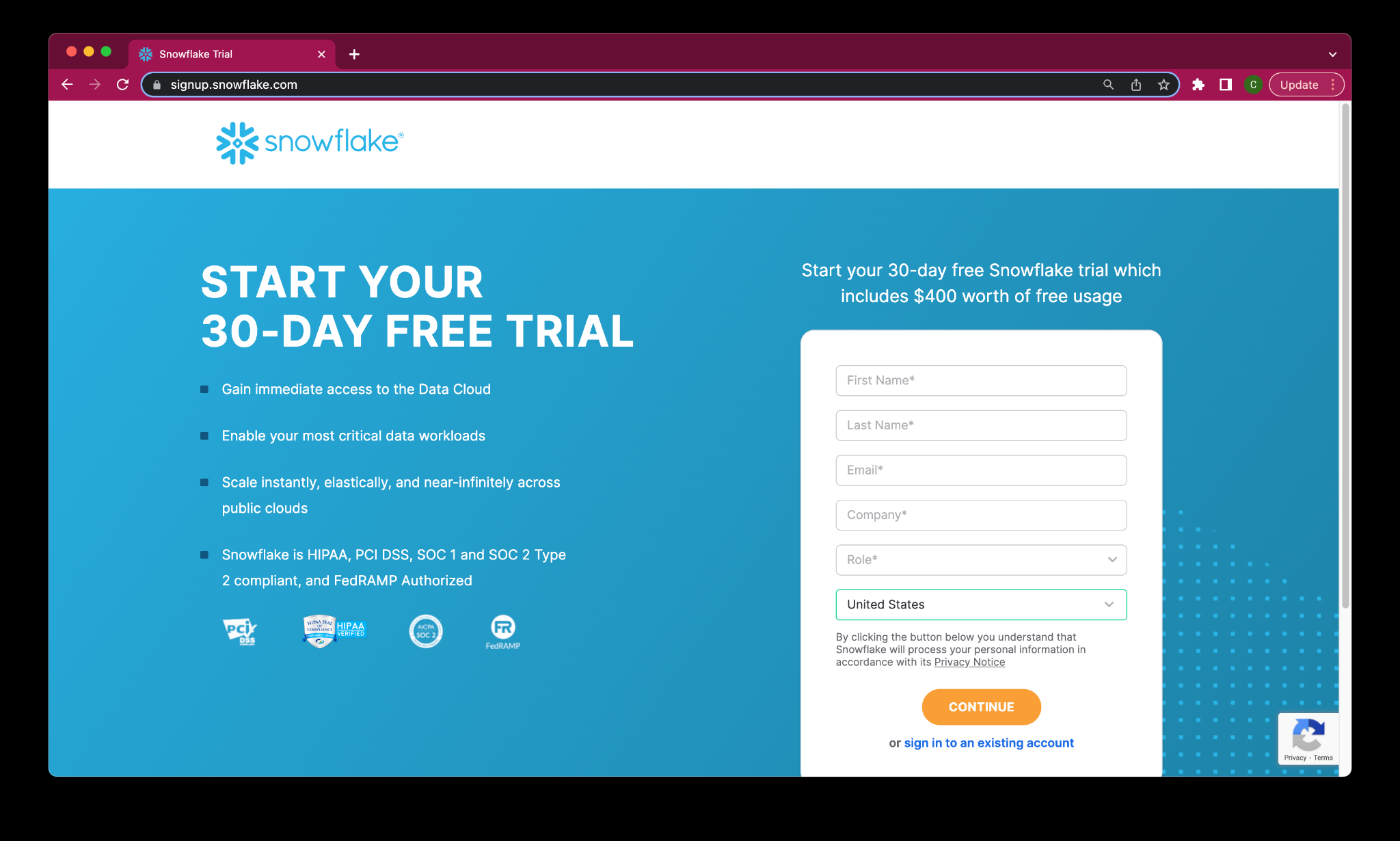
Fill out the Snowflake trial account form here. Use an email address that is not associated with an existing Snowflake account.
When signing up for your Snowflake account, select the region that is physically closest to you and choose Enterprise as your Snowflake edition. Please note that the Snowflake edition, cloud provider, and region used when following this guide do not matter.
After registering, you will receive an email from Snowflake with an activation link and URL for accessing your trial account. Finish setting up your account following the instructions in the email.

Step 2: Create a Coalesce Trial Account with Snowflake Partner Connect

Once you are logged into your Snowflake account, sign up for a free Coalesce trial account using Snowflake Partner Connect. Check your Snowflake account profile to make sure that it contains your fist and last name.

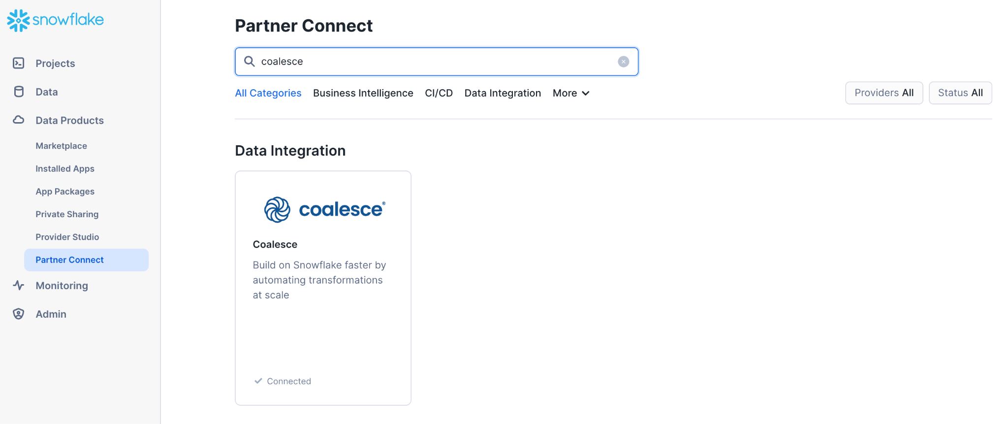
Select Data Products > Partner Connect in the navigation bar on the left hand side of your screen and search for Coalesce in the search bar.
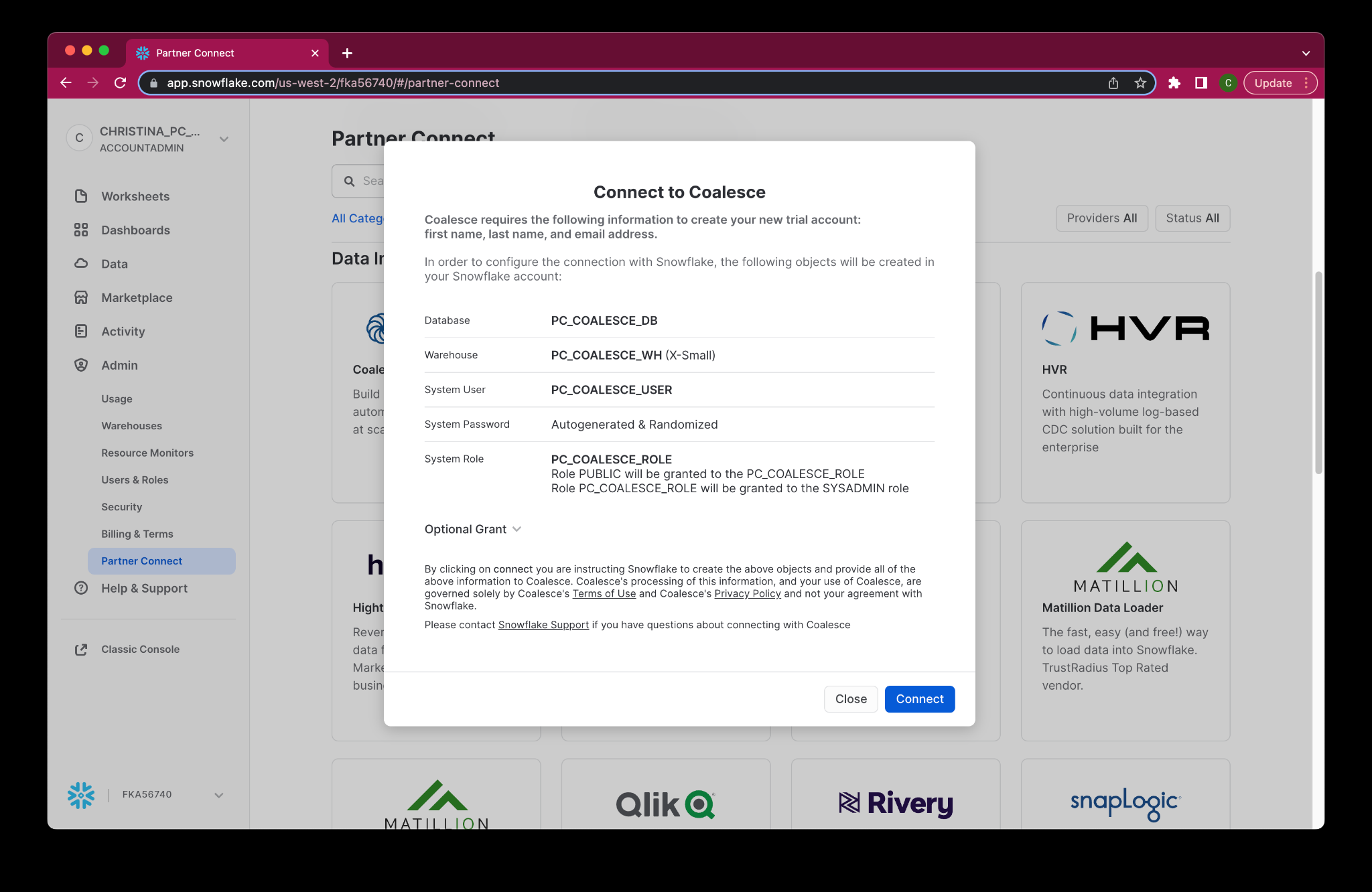
Review the connection information and then click Connect.
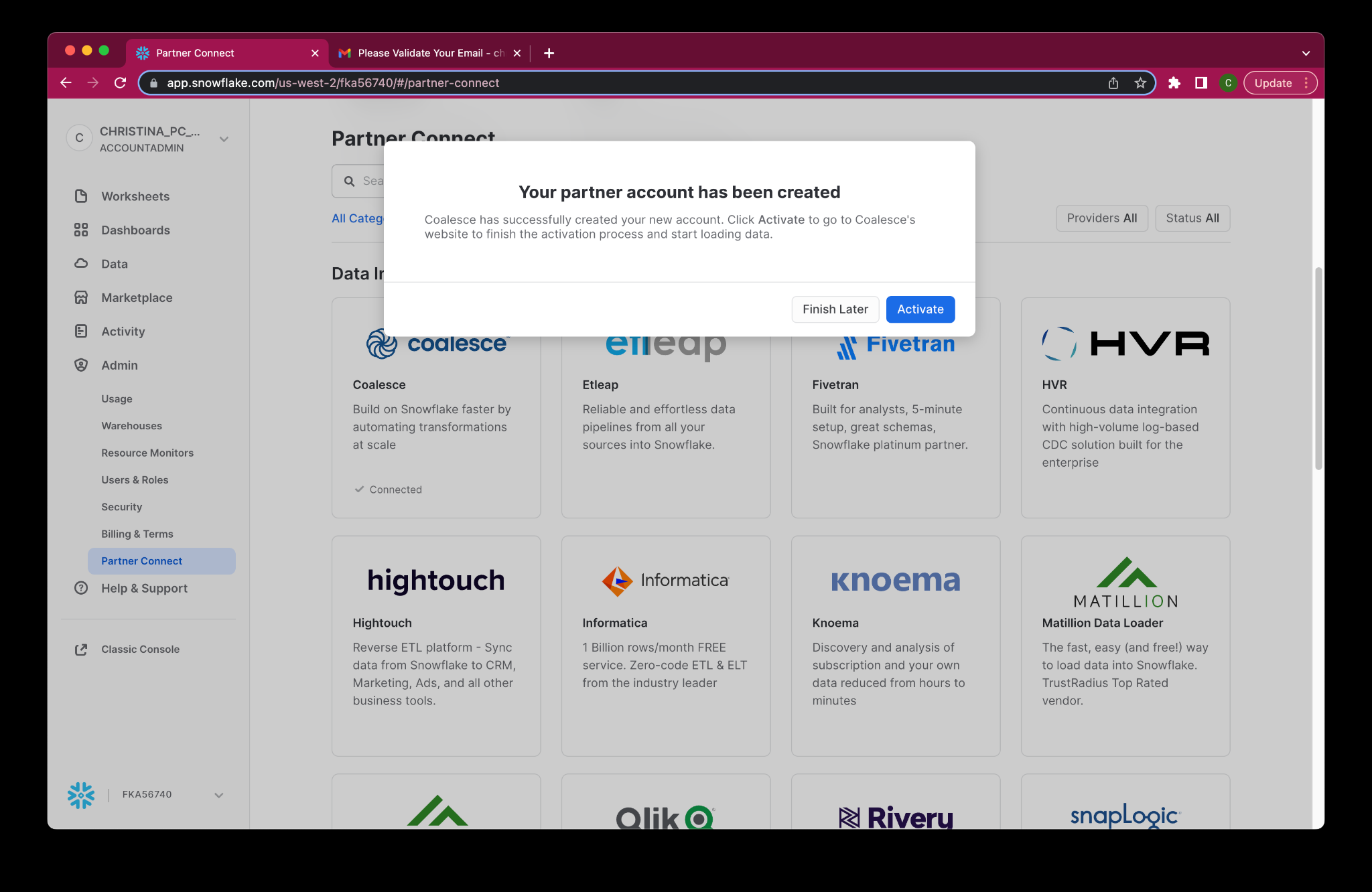
When prompted, click Activate to activate your account. You can also activate your account later using the activation link emailed to your address.
Once you’ve activated your account, fill in your information to complete the activation process.

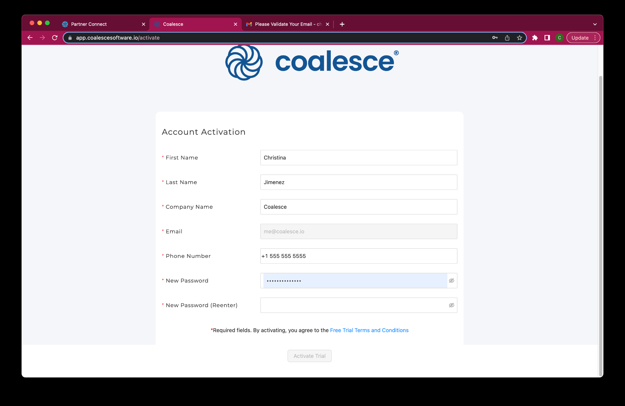
Congratulations! You’ve successfully created your Coalesce trial account.

Step 3: Set Up The Dataset

We will be using a M Warehouse size within Snowflake for this lab. You can upgrade this within the admin tab of your Snowflake account.
In your Snowflake account, click on the Worksheets Tab in the left-hand navigation bar.
Within Worksheets, click the "+" button in the top-right corner of Snowsight and choose "SQL Worksheet.”
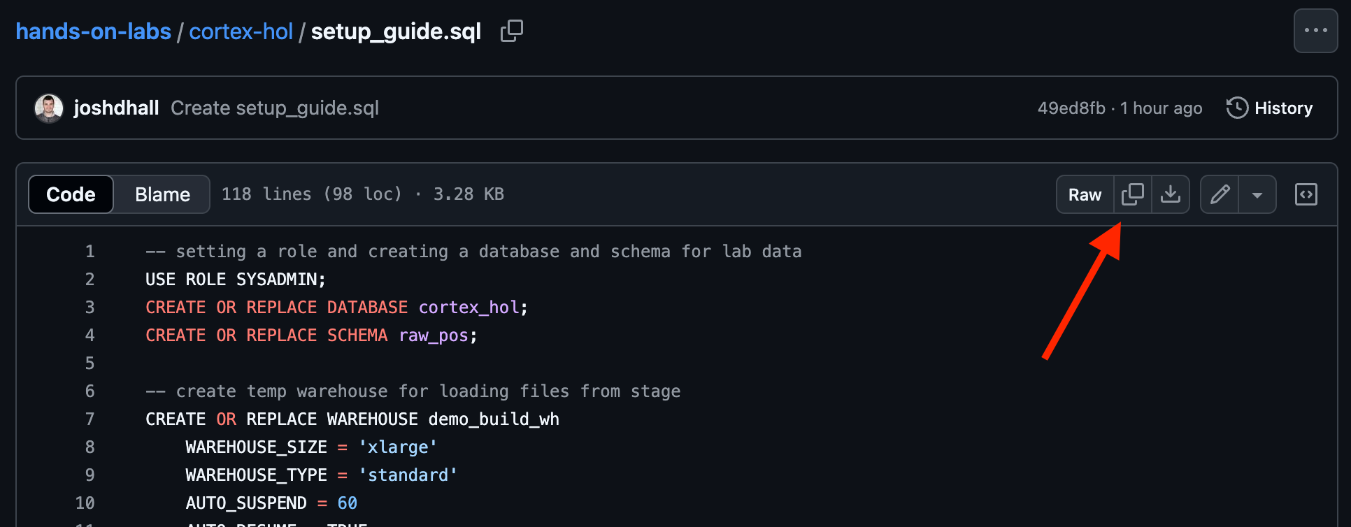
Navigate to the Cortex HOL Data Setup File that is hosted on GitHub.
Within GitHub, navigate to the right side and click "Copy raw contents". This will copy all of the required SQL into your clipboard.
Paste the setup SQL from GitHub into your Snowflake Worksheet. Then click inside the worksheet and select All (CMD + A for Mac or CTRL + A for Windows) and Click "► Run".
After clicking "► Run" you will see queries begin to execute. These queries will run one after another with the entire worksheet taking around 5 minutes. Upon completion you will see a message that states your HOL data setup is now complete.

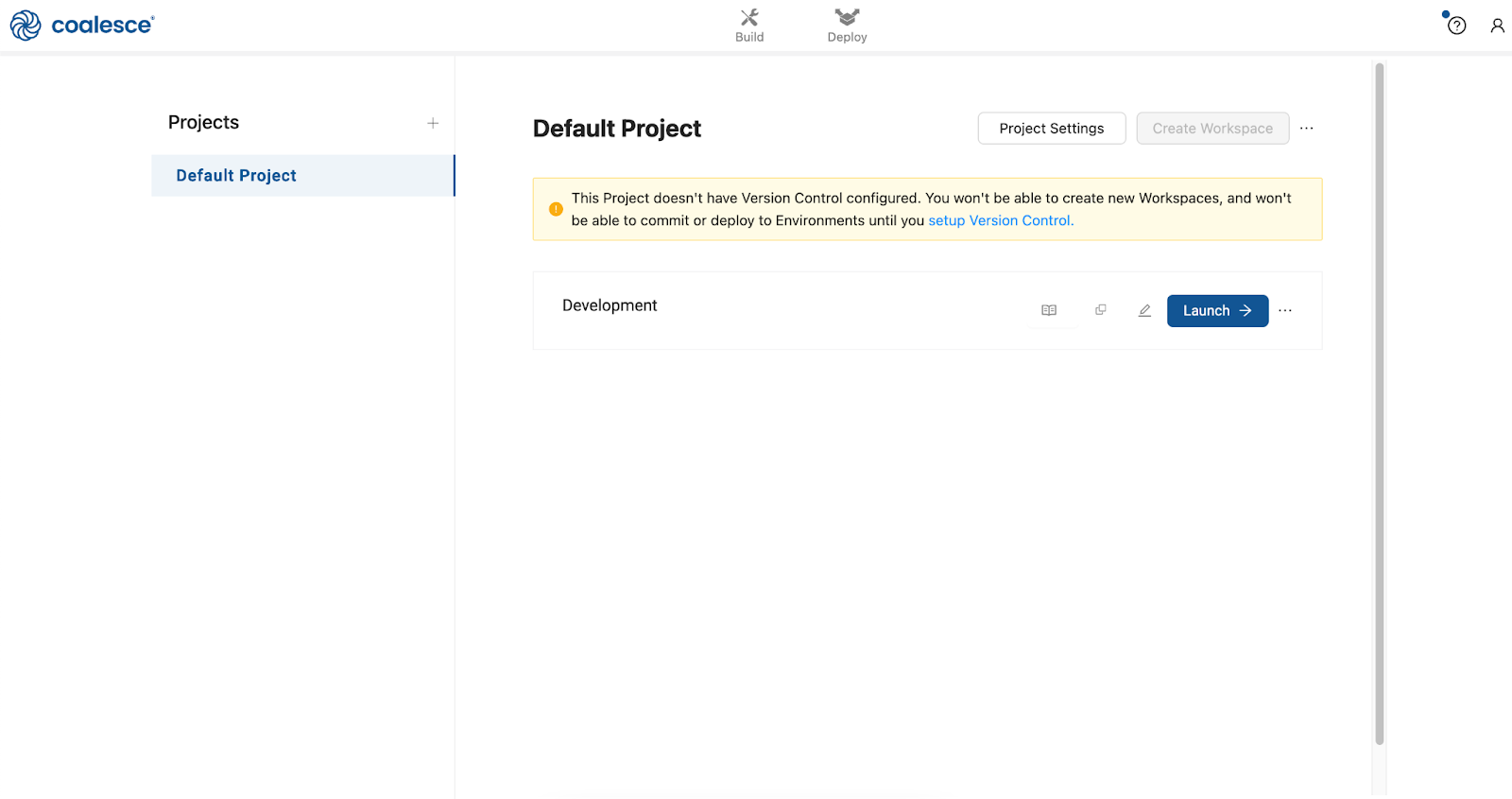
Once you’ve activated your Coalesce trial account and logged in, you will land in your Projects dashboard. Projects are a useful way of organizing your development work by a specific purpose or team goal, similar to how folders help you organize documents in Google Drive.

Your trial account includes a default Project to help you get started. Click on the Launch button next to your Development Workspace to get started.

Step 4: Add the Cortex Package from the Coalesce Marketplace

You will need to add the ML Forecast node into your Coalesce workspace in order to complete this lab.

Launch your workspace within your Coalesce account
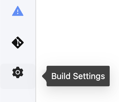
Navigate to the build settings in the lower left hand corner of the left sidebar
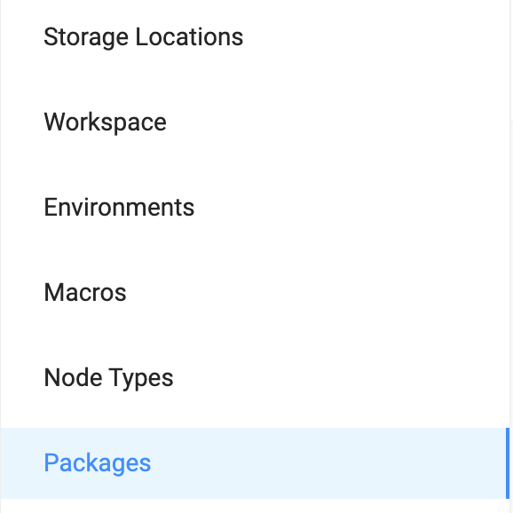
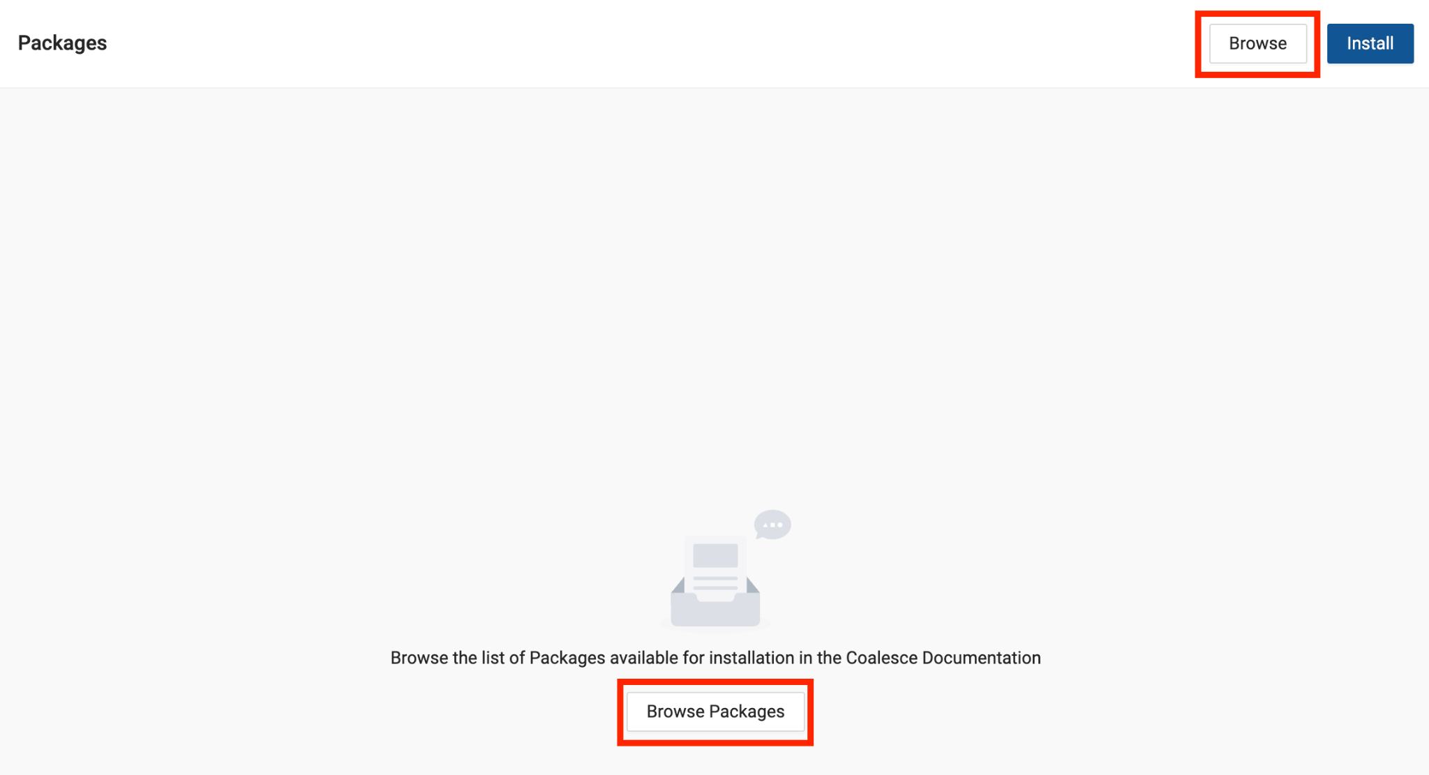
Select Packages from the Build Settings options
Select Browse to Launch the Coalesce Marketplace
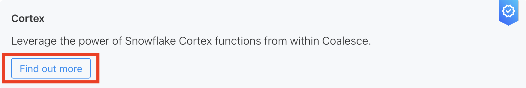
Select Find out more within the Cortex package
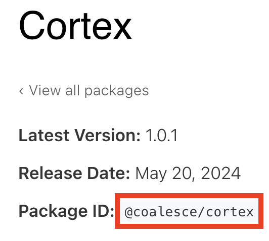
Copy the package ID from the Cortex page
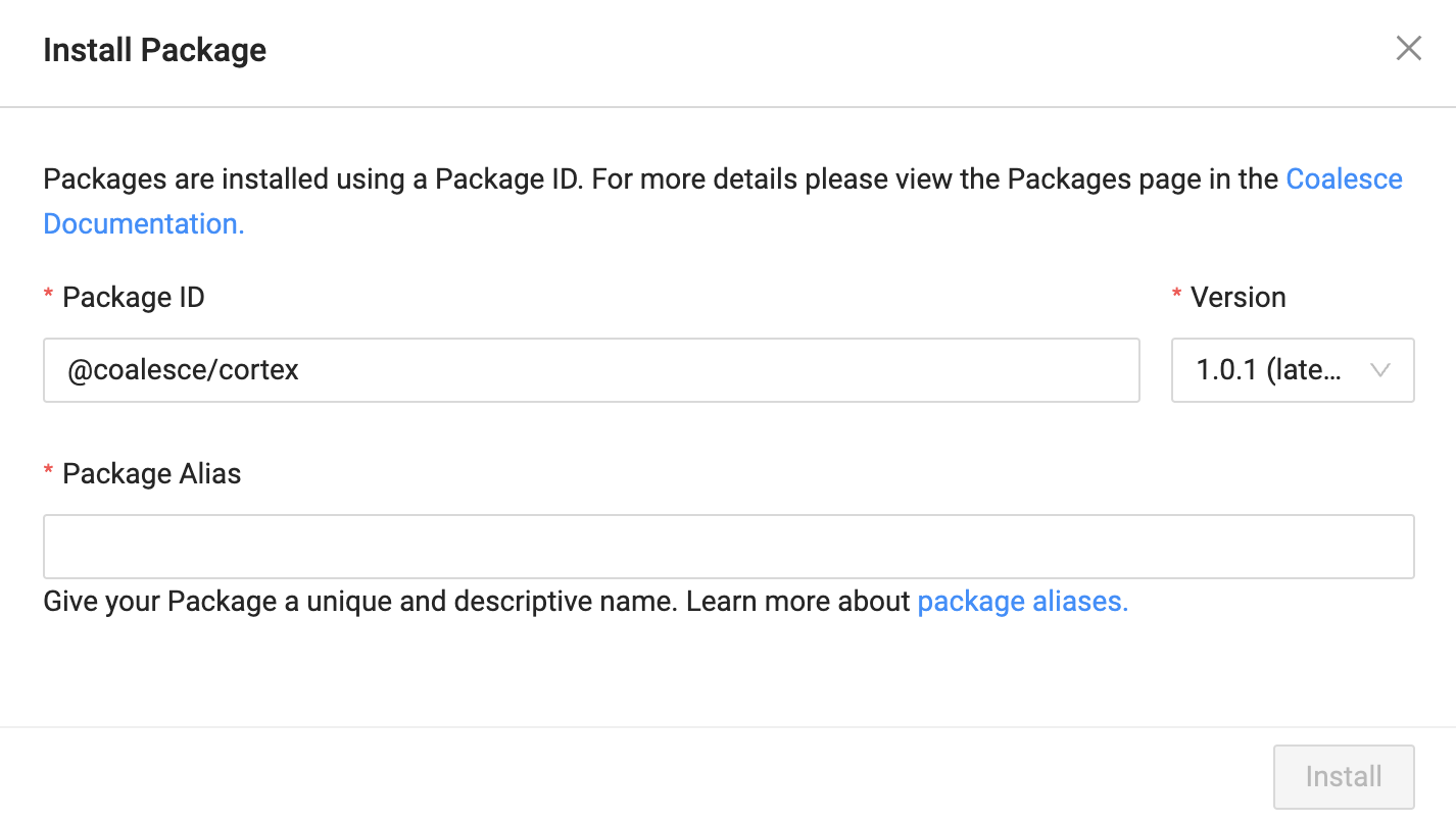
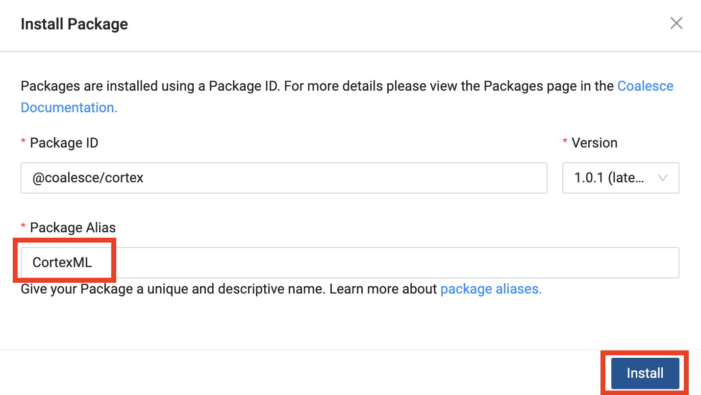
Back in Coalesce, select the Install button:
Paste the Package ID into the corresponding input box:
Give the package an Alias, which is the name of the package that will appear within the Build Interface of Coalesce. And finish by clicking Install.

Navigating the Coalesce User Interface

About this lab: Screenshots (product images, sample code, environments) depict examples and results that may vary slightly from what you see when you complete the exercises. This lab exercise does not include Git (version control). Please note that if you continue developing in your Coalesce account after this lab, none of your work will be saved or committed to a repository unless you set up before developing.

Let's get familiar with Coalesce by walking through the basic components of the user interface.

Once you've activated your Coalesce trial account and logged in, you will land in your Projects dashboard. Projects are a useful way of organizing your development work by a specific purpose or team goal, similar to how folders help you organize documents in Google Drive.

Your trial account includes a default Project to help you get started.

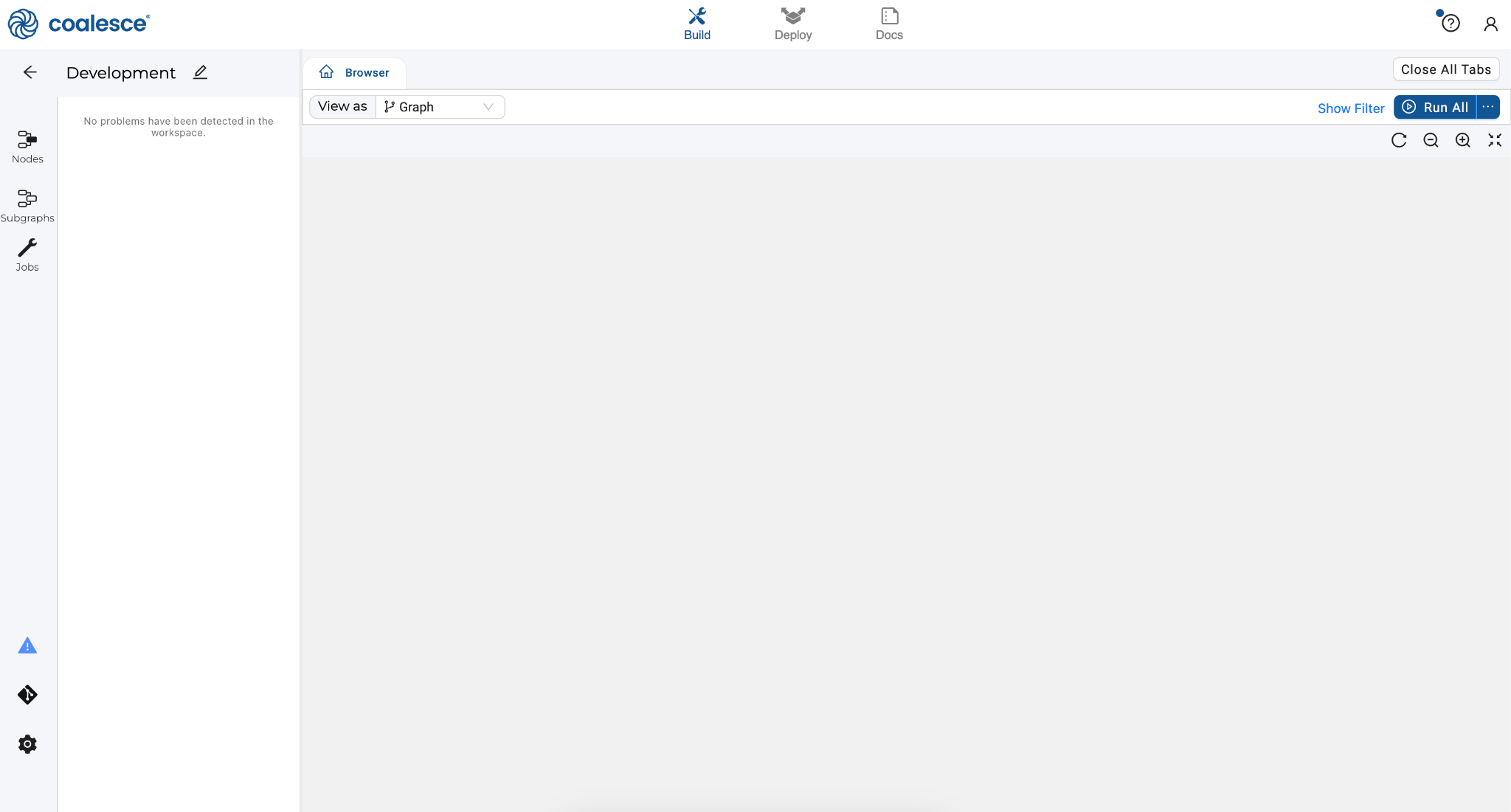
Launch your Development Workspace by clicking the Launch button and navigate to the Build Interface of the Coalesce UI. This is where you can create, modify and publish nodes that will transform your data.

Nodes are visual representations of objects in Snowflake that can be arranged to create a Directed Acyclic Graph (DAG or Graph). A DAG is a conceptual representation of the nodes within your data pipeline and their relationships to and dependencies on each other.
In the Browser tab of the Build interface, you can visualize your node graph using the Graph, Node Grid, and Column Grid views. In the upper right hand corner, there is a person-shaped icon where you can manage your account and user settings.
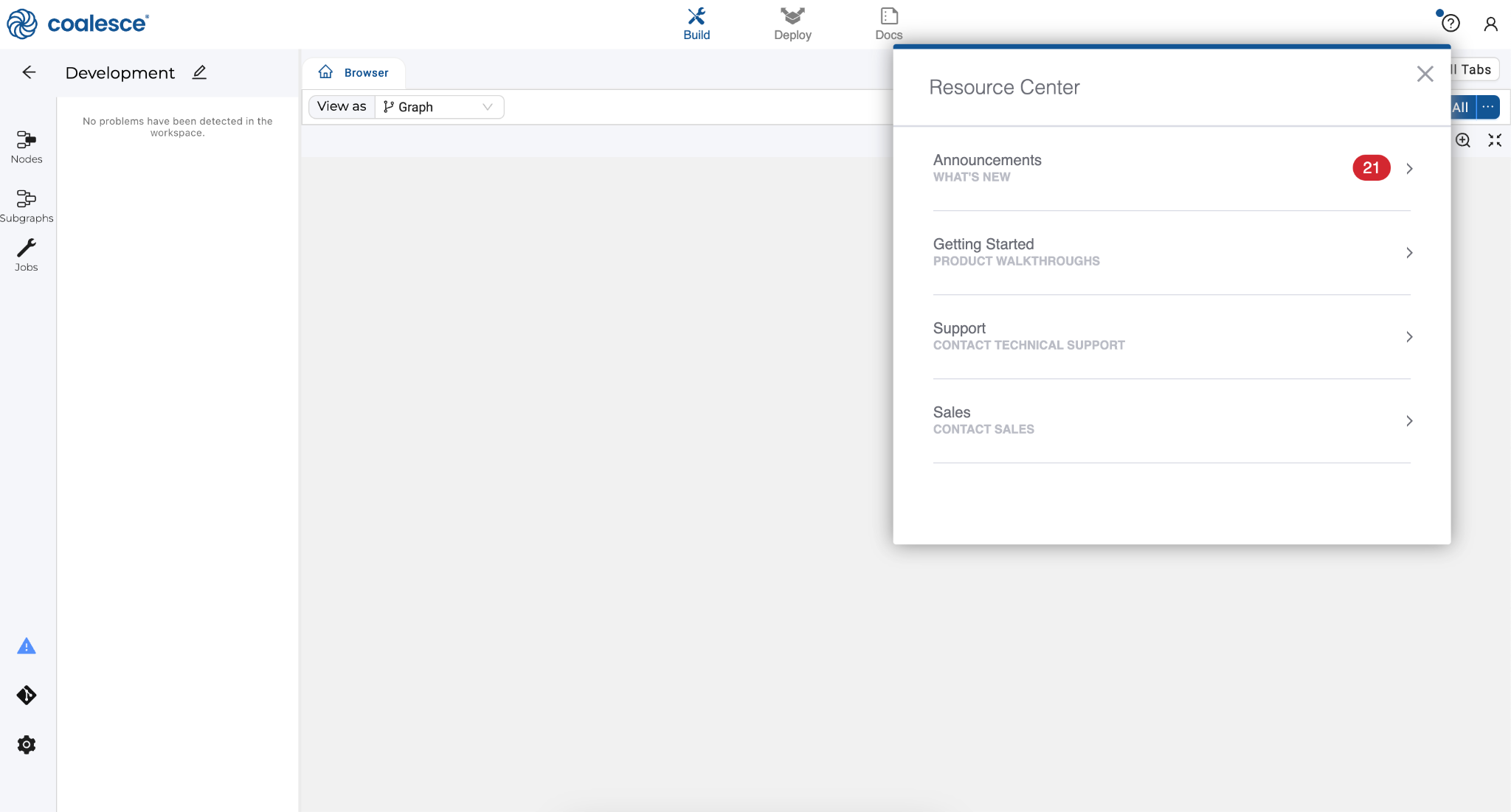
By clicking the question mark icon, you can access the Resource Center to find product guides, view announcements, request support, and share feedback.
The Browser tab of the Build interface is where you’ll build your pipelines using nodes. You can visualize your graph of these nodes using the Graph, Node Grid, and Column Grid views. While this area is currently empty, we will build out nodes and our Graph in subsequent steps of this lab.
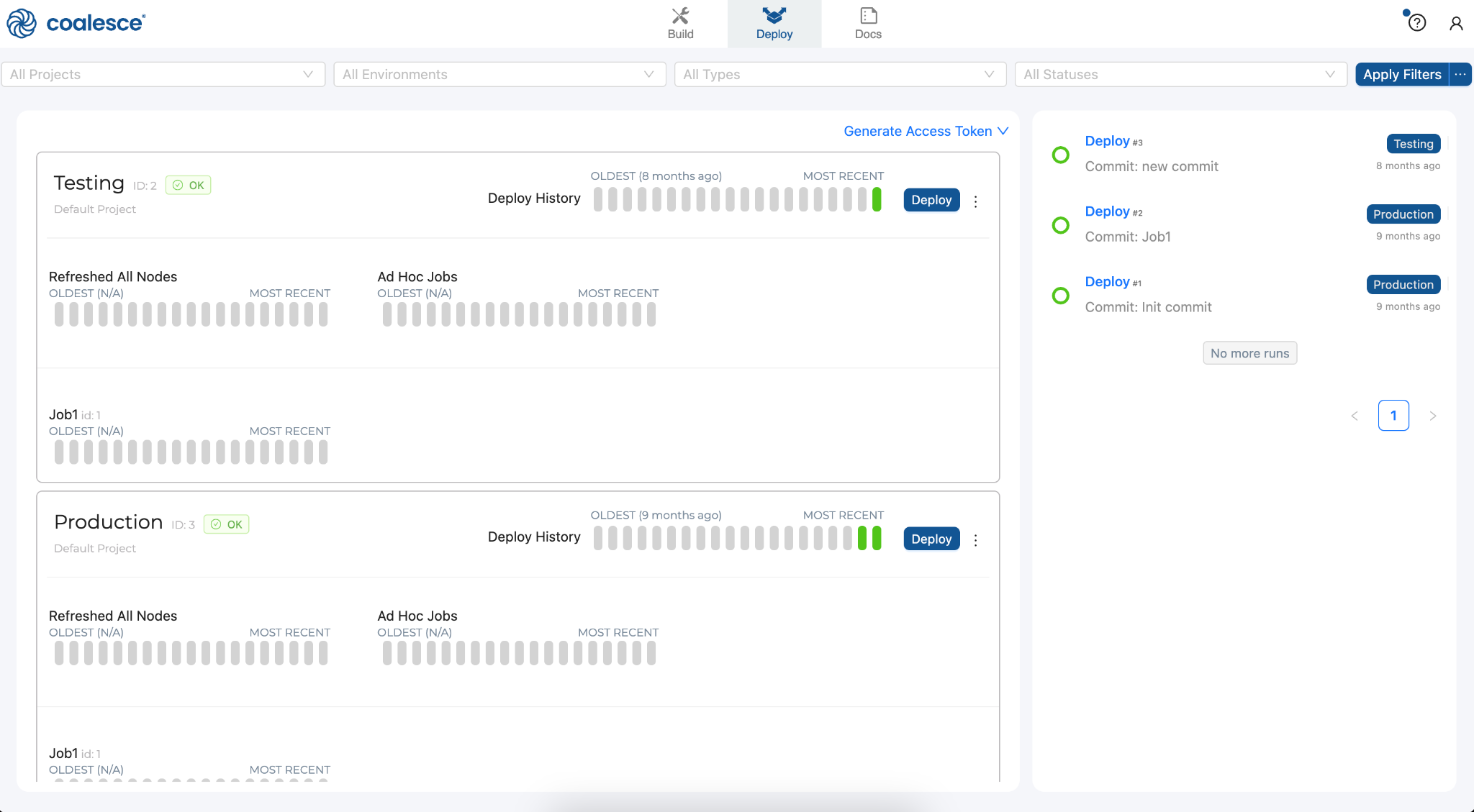
Next to the Build page is the Deploy page. This is where you will push your pipeline to other environments such as Testing or Production.
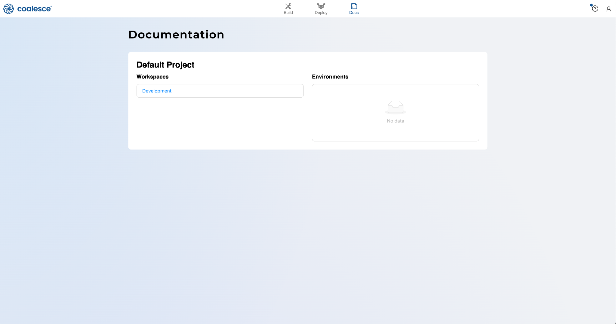
Next to the Deploy page is the Docs page. Documentation is an essential step in building a sustainable data architecture, but is sometimes put aside to focus on development work to meet deadlines. To help with this, Coalesce automatically generates and updates documentation as you work.

Configure Storage Locations and Mappings

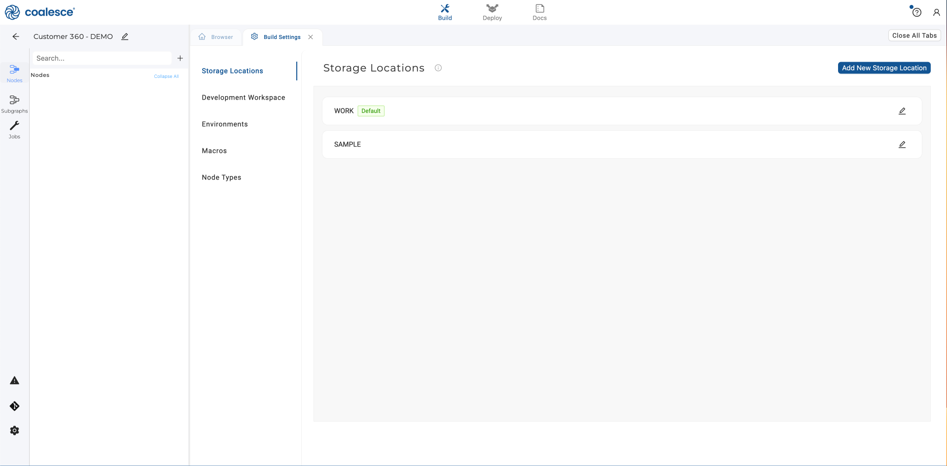
Before you can begin transforming your data, you will need to configure storage locations. Storage locations represent a logical destination in Snowflake for your database objects such as views and tables.

To add storage locations, navigate to the left side of your screen and click on the Build settings cog.
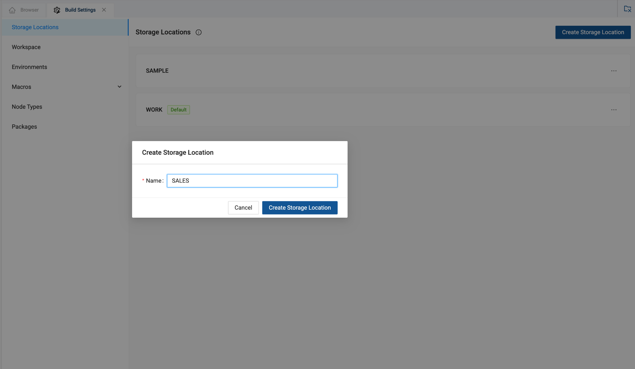
Click the “Add New Storage Locations” button and name it SALES for your raw customer data.
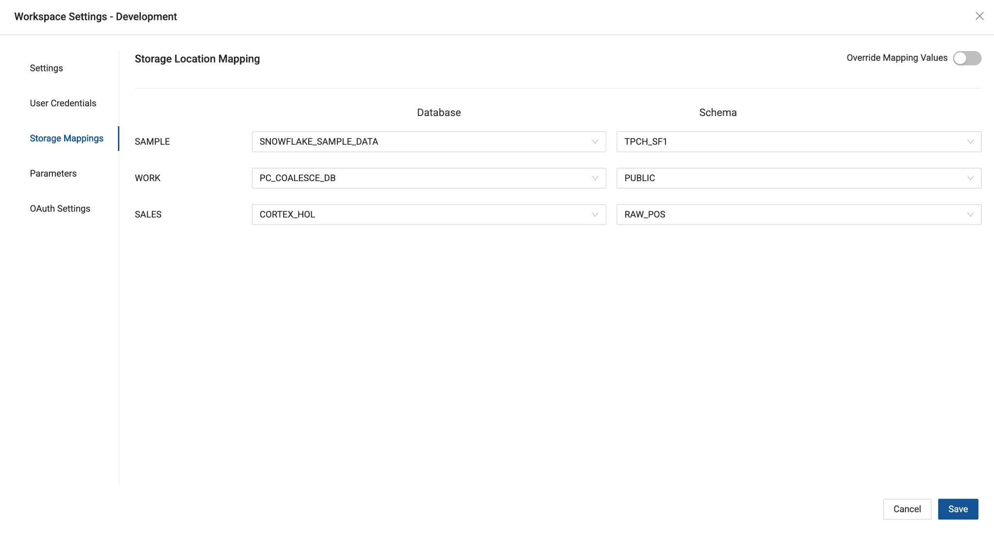
Now map your storage location to their logical destinations in Snowflake. In the upper left corner next to your Workspace name, click on the pencil icon to open your Workspace settings. Click on Storage Mappings and map your SALES location to the CORTEX_HOL database and the RAW_POS schema. Select Save to ensure Coalesce stores your mappings.
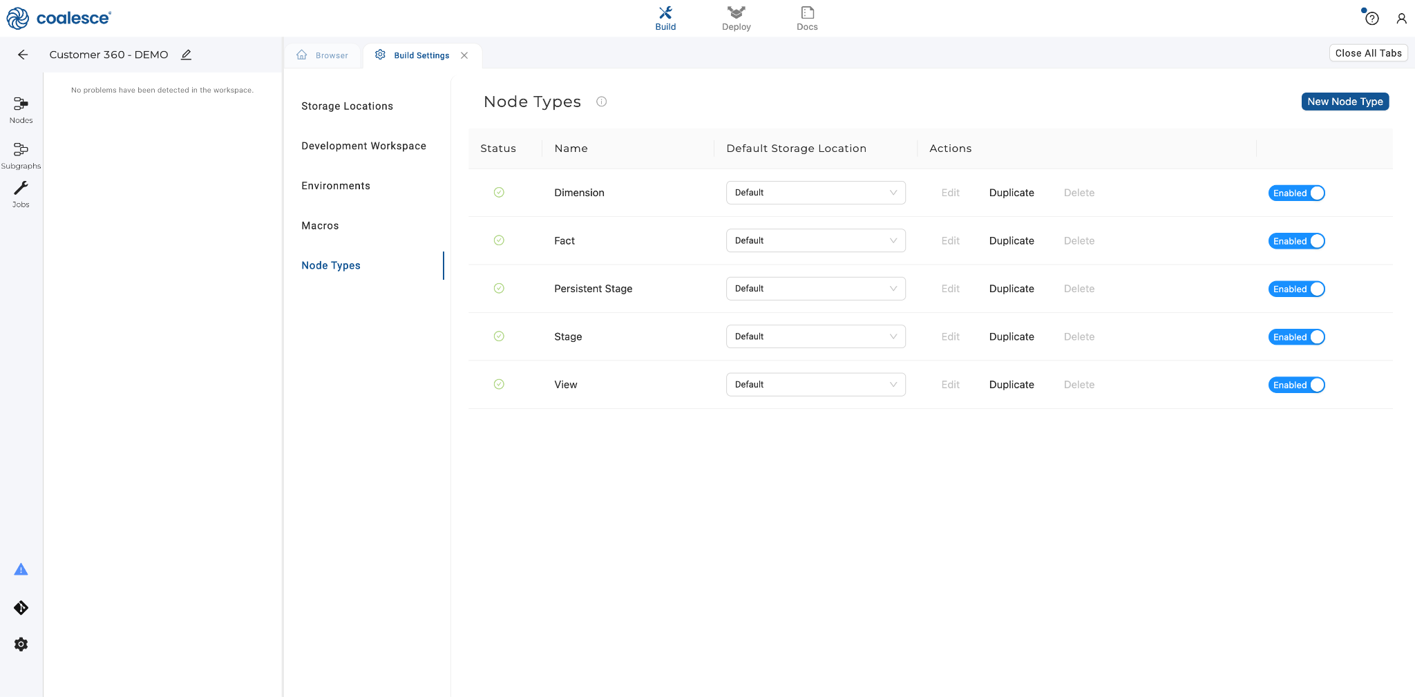
Go back to the build settings and click on Node Types and then click the toggle button next to View to enable View node types. Now you’re ready to start building your pipeline.

Adding Data Sources

Let’s start to build the foundation of your data pipeline by creating a Graph (DAG) and adding data in the form of Source nodes.

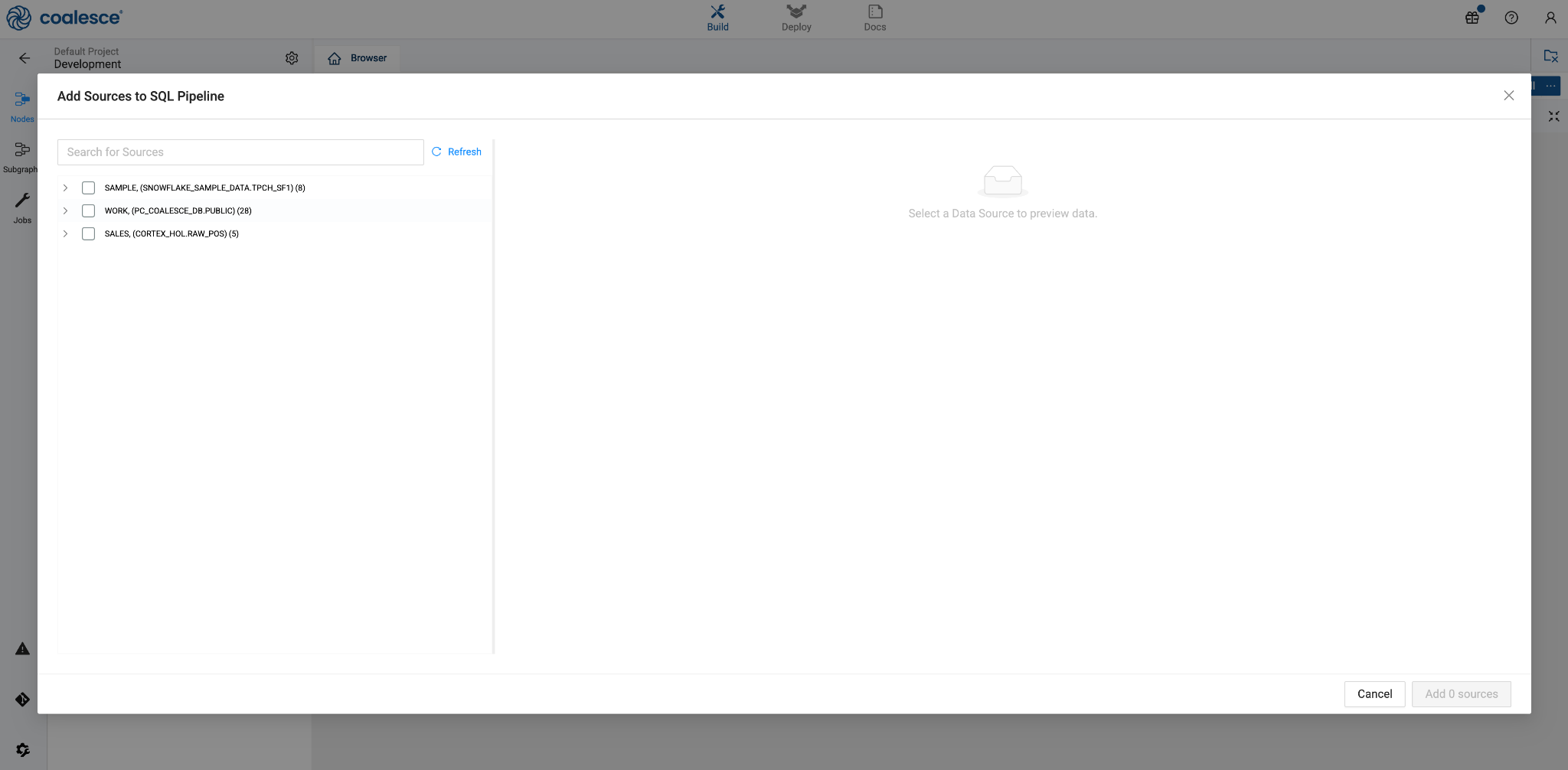
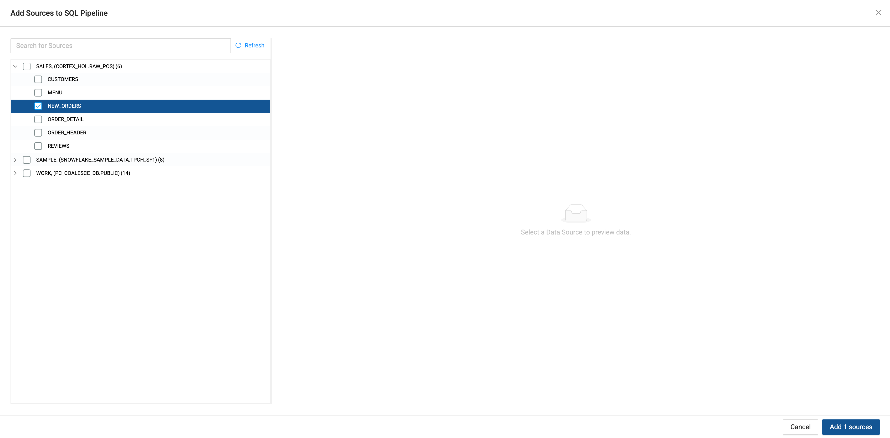
Start in the Build interface and click on Nodes in the left sidebar (if not already open). Click the + icon and select Add Sources.
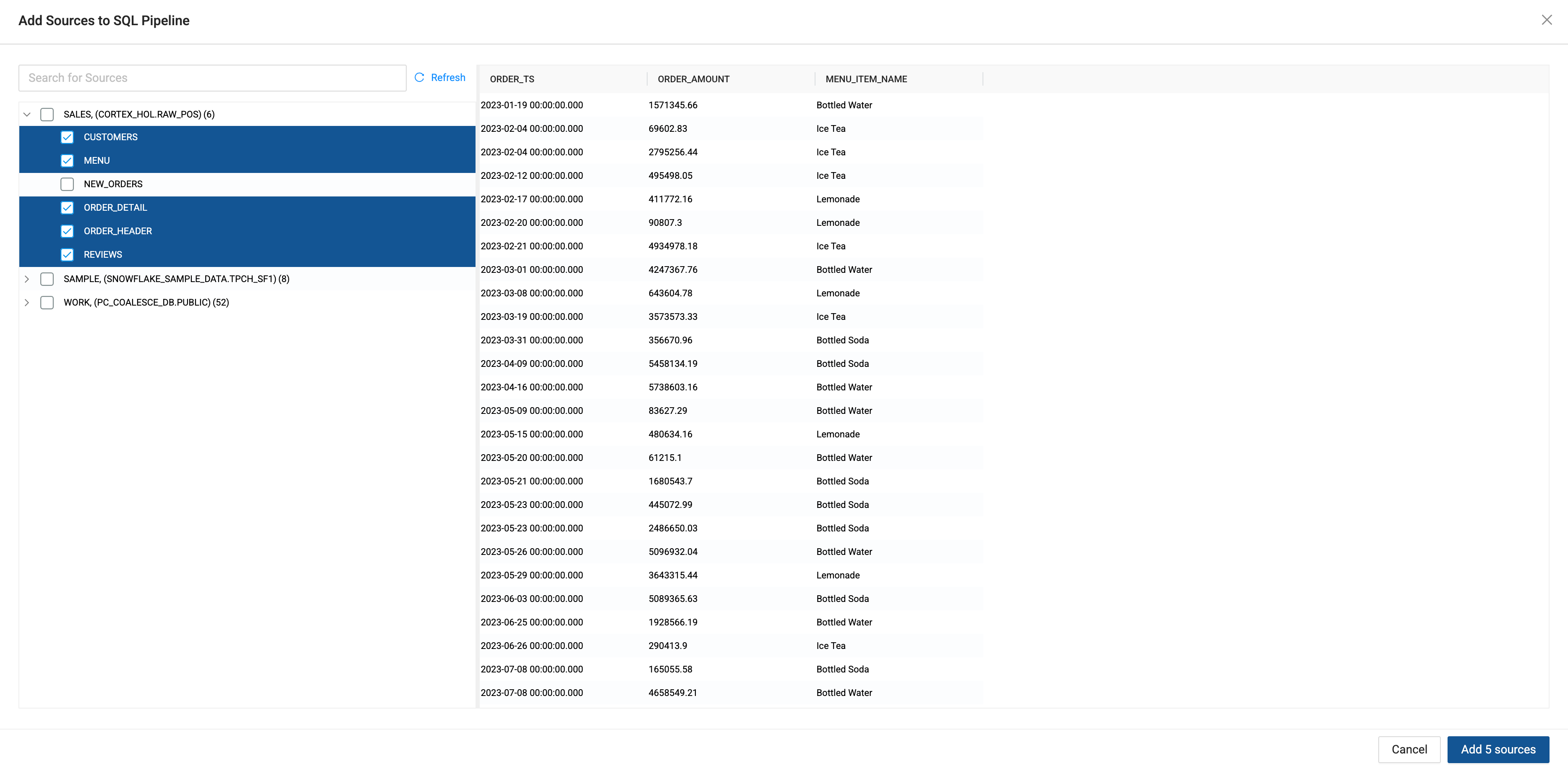
Select all of the tables from the SALES storage location. You can click on the check box next to the storage location name to select all of the tables.
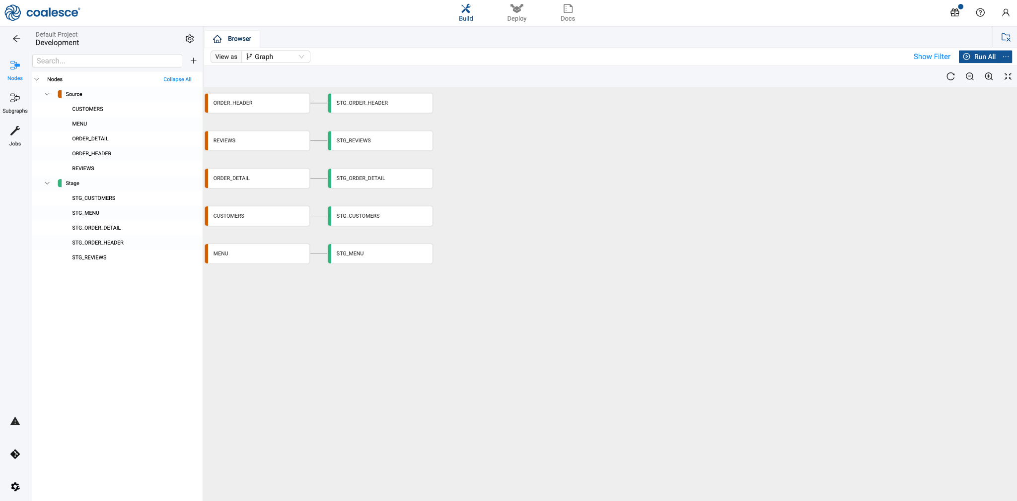
You'll now see your graph populated with your Source nodes. Note that they are designated in red. Each node type in Coalesce has its own color associated with it, which helps with visual organization when viewing a Graph.
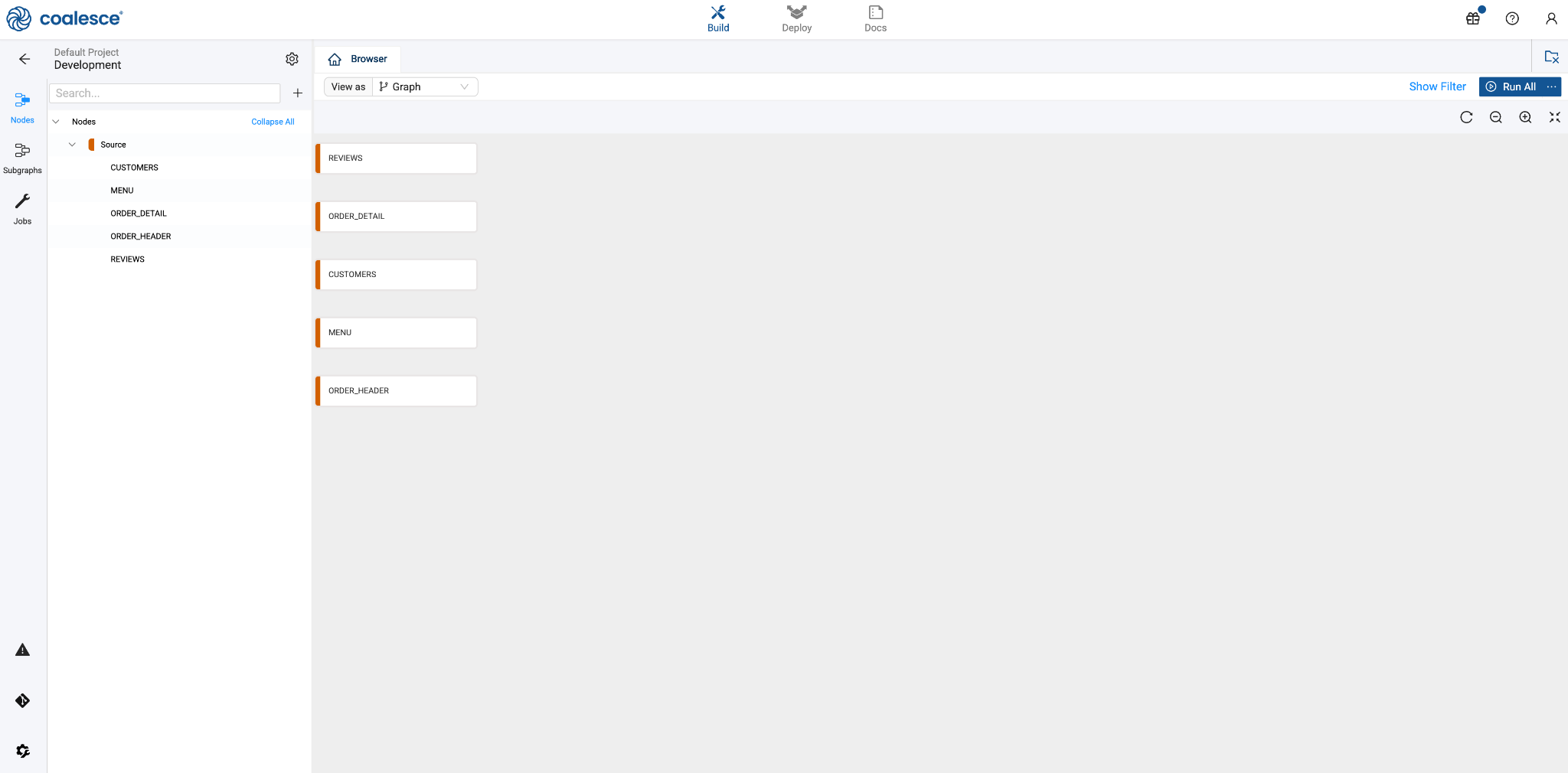
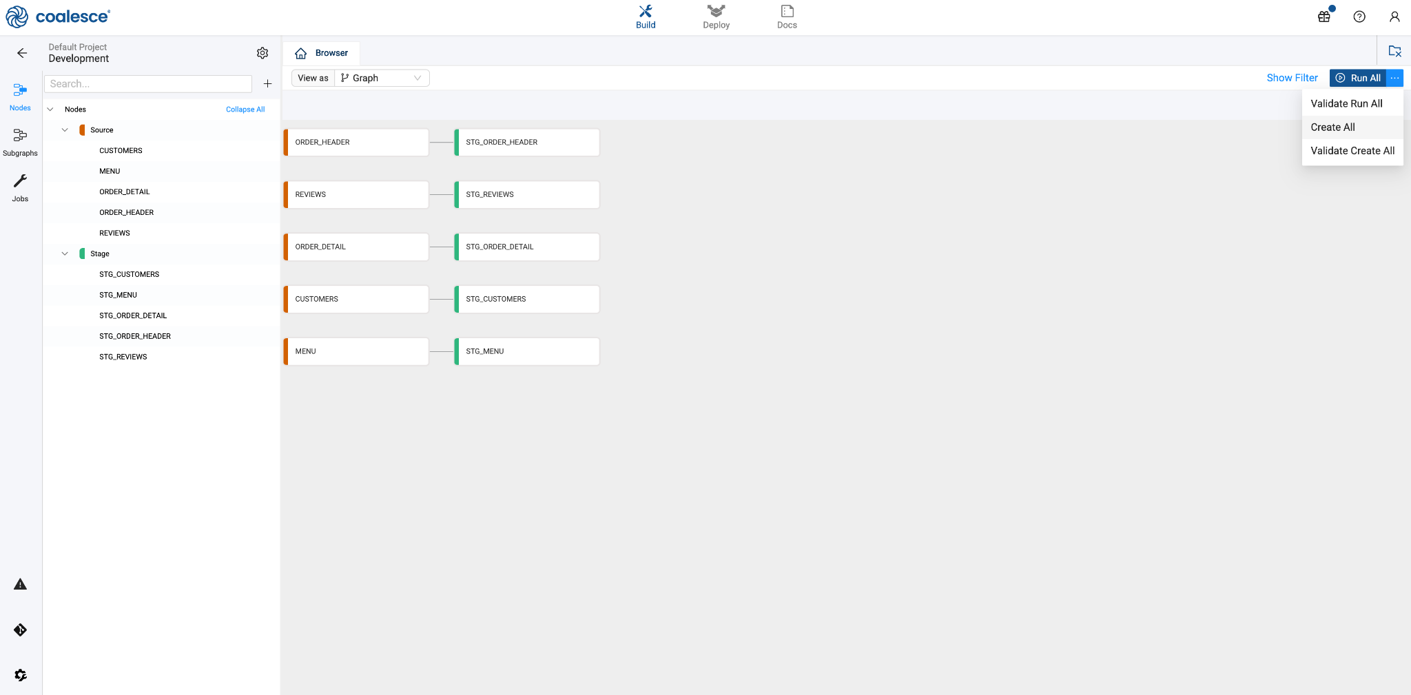
Select Create All and Run All to create and populate the tables as objects in Snowflake.

Creating Stage Nodes

Now that you’ve added your Source nodes, let’s prepare the data by adding business logic with Stage nodes. Stage nodes represent staging tables within Snowflake where transformations can be previewed and performed. Let's start by adding a standardized "stage layer" for all sources.

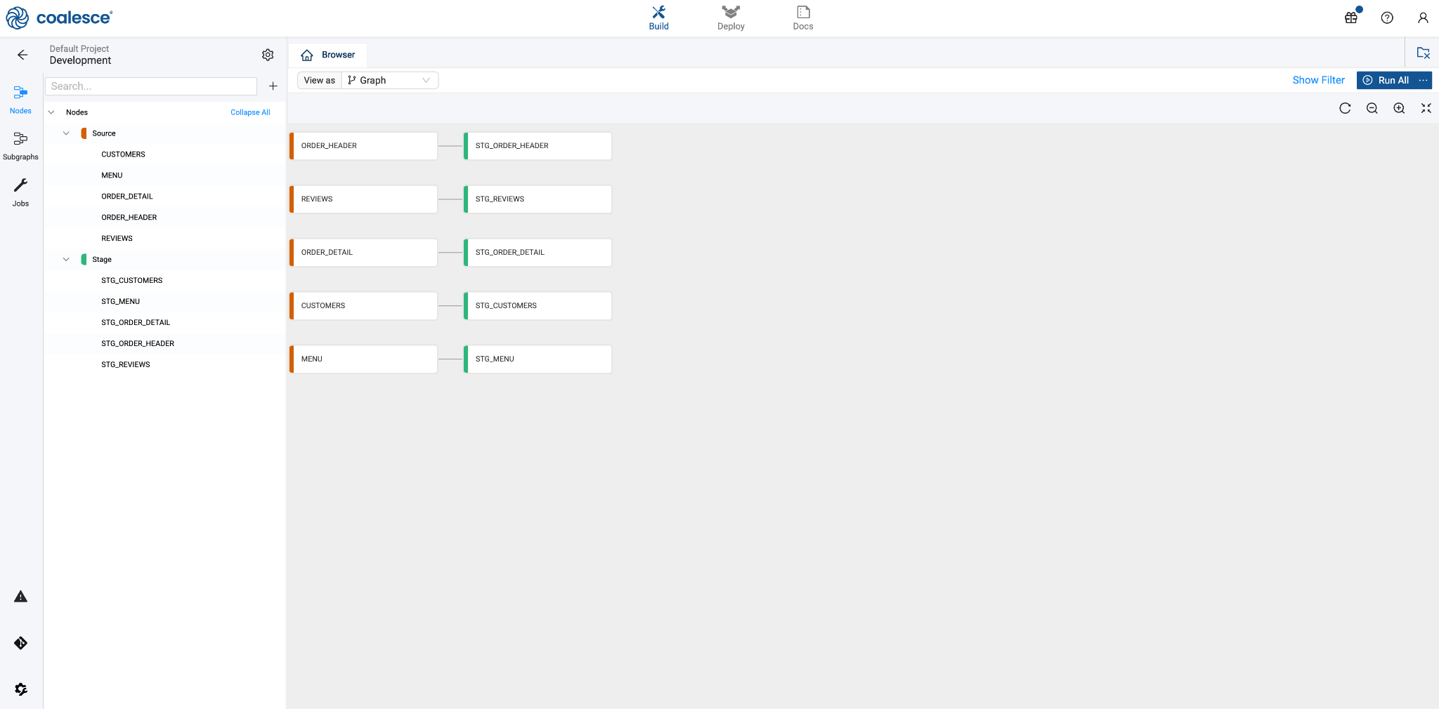
Press and hold the Shift key to multi-select all of your Source nodes from the node pane on the left side of your screen. Then right click and select Add Node > Stage from the drop down menu. You will now see that all of your Source nodes have corresponding Stage tables associated with them. If the 14M/38M data sources are being used, drop that suffix in the Node name in this case STG_ORDER_HEADER
Now change the Graph to a Column Grid by using the top left dropdown menu. By using the Column Grid view, you can search and group by different column headers.
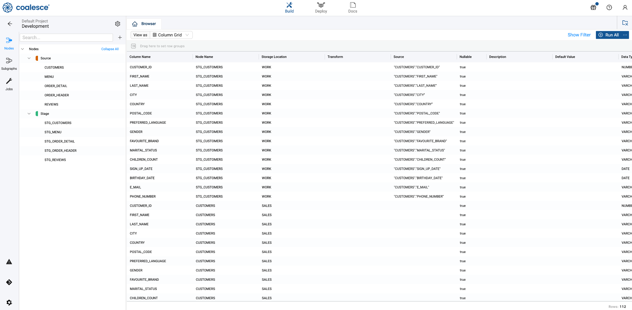
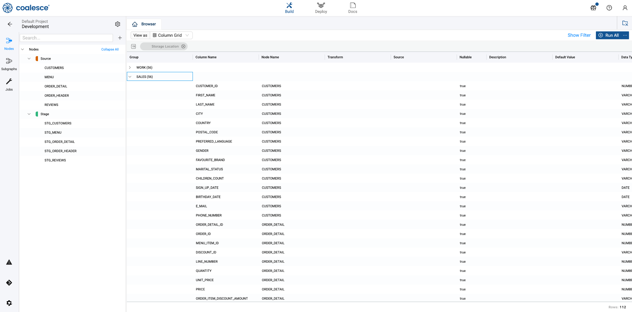
Click on the Storage Location header and drag it to the sorting bar below the View As dropdown menu. You have now grouped your rows by Storage Location. Then expand all the columns from your SALES location.
Change back to the Graph view from Column Grid to with the dropdown menu.
Now let’s create the foundation for your data pipeline. In the upper right hand corner, press the Create All button to create your tables in Snowflake. Then click the Run All button to populate your nodes with data.

Exploring the Node Editor

Your Node Editor is used to edit the node object, the columns within it, and its relationship to other nodes. There are a few different components to the Node Editor.

Double click on your STG_CUSTOMER node to open up your Node Editor. The large middle section is your Mapping grid, where you can see the structure of your node along with column metadata like transformations, data types, and sources.
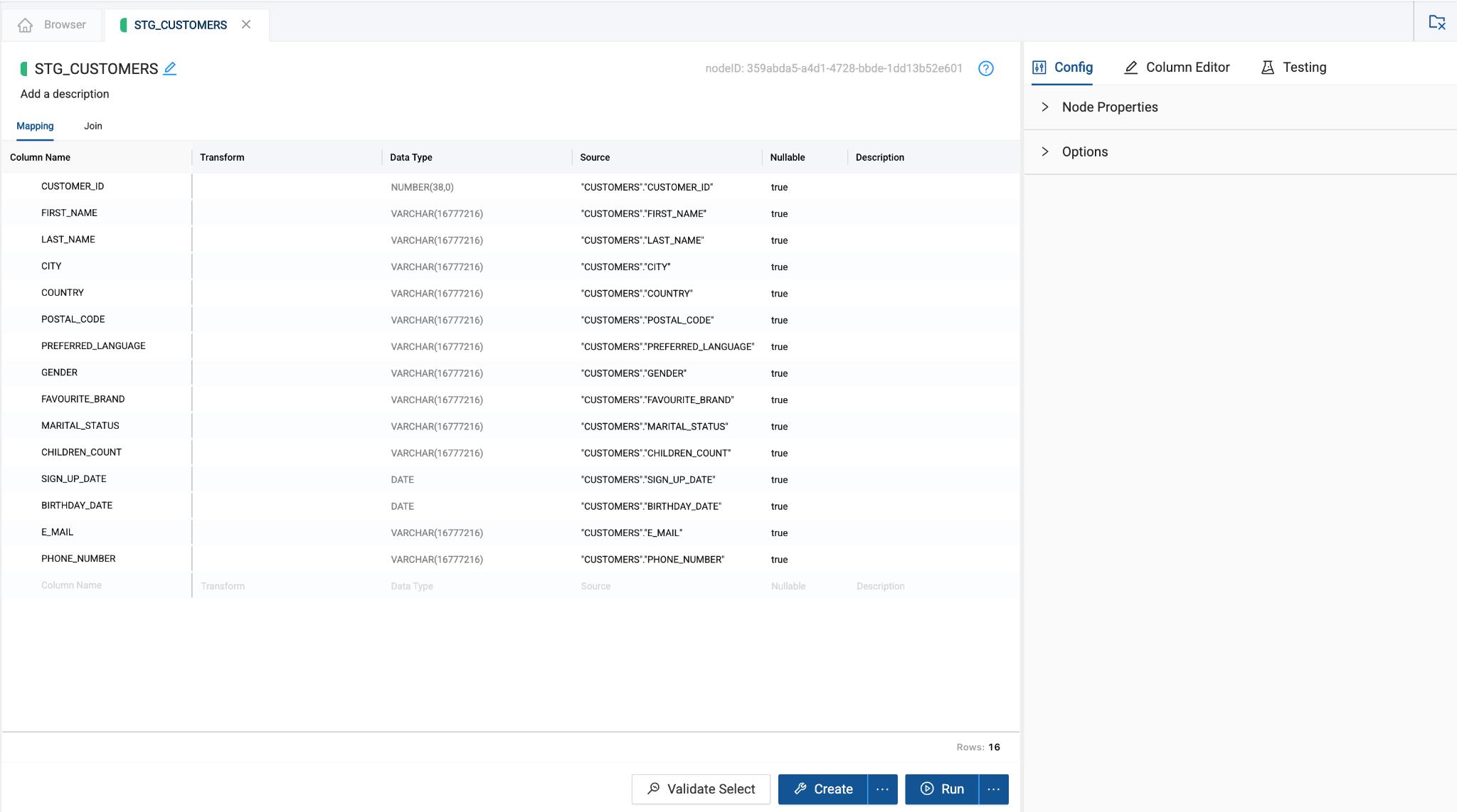
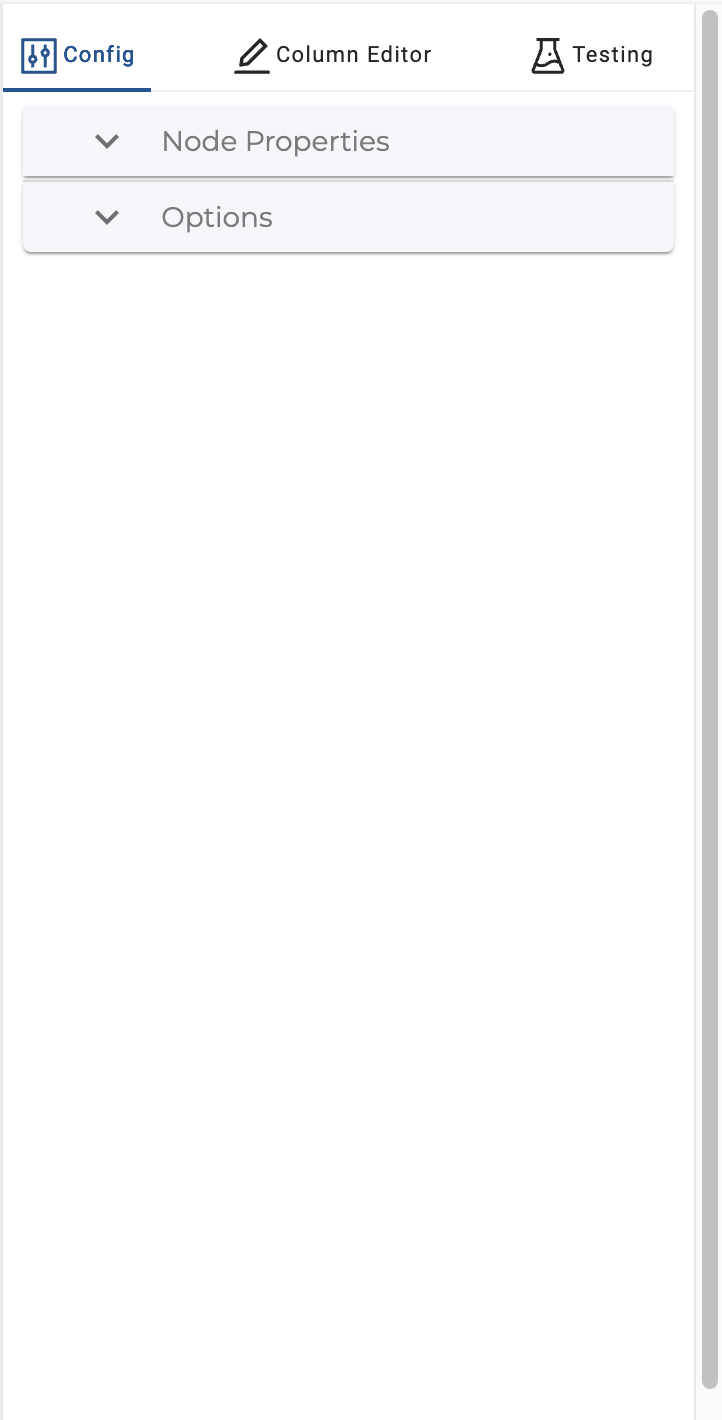
On the right hand side of the Node Editor is the Config section, where you can view and set configurations based on the type of node you’re using.
At the bottom of the Node Editor, press the arrow button to view the Data Preview pane.

Applying Single Column Transformations

Now let’s apply a single column transformation in your STG_CUSTOMER node by applying a consistent naming convention to our customer names. This will ensure that any customer names are standardized.

Select the FIRST_NAME column and click the blank Transform field in the Mapping grid. Enter the following transformation and then press Enter:
```
UPPER({{SRC}})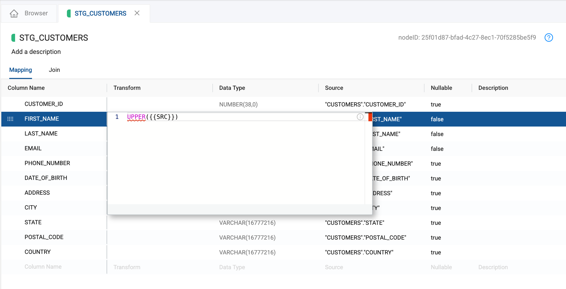
```
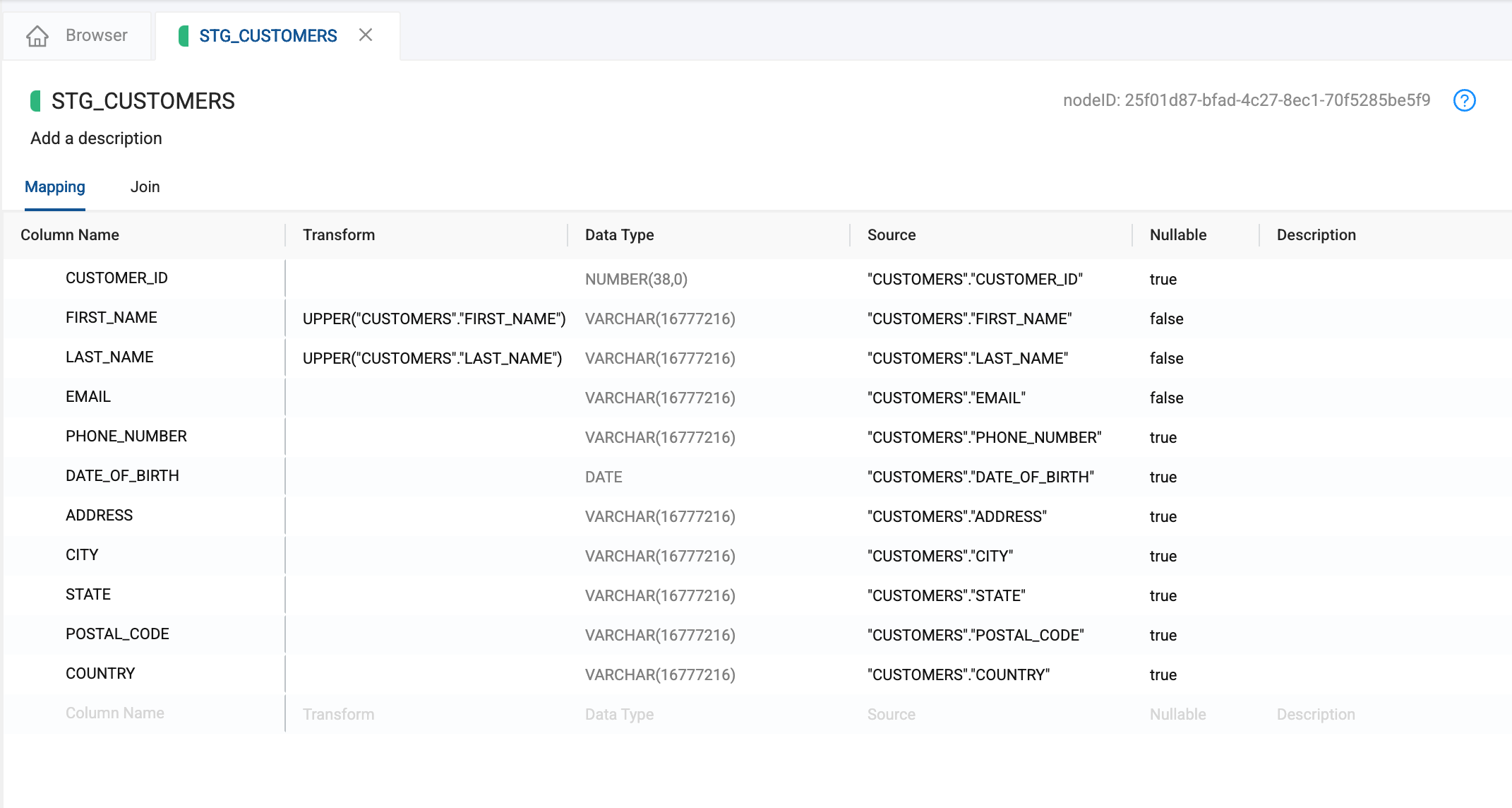
Repeat this transformation for your LAST_NAME column:
```
UPPER({{SRC}})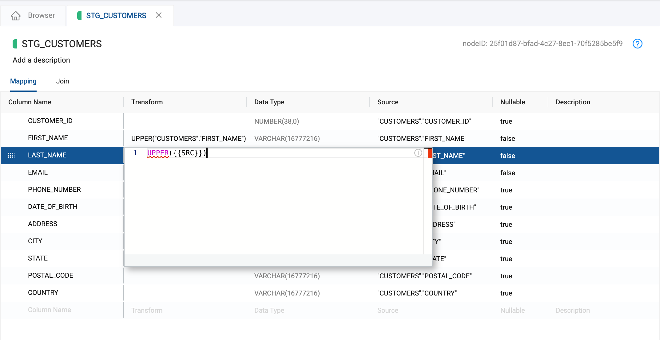
```
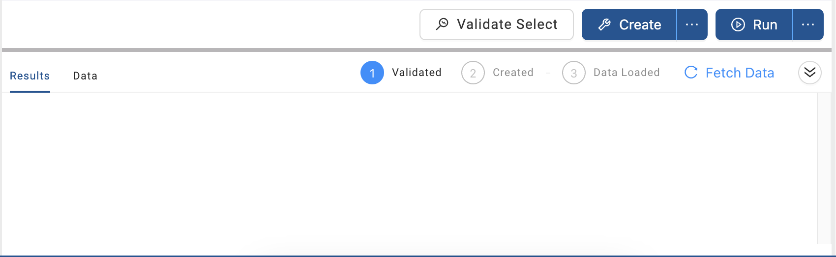
Click the Create and Run buttons to create and repopulate your node.

Joining Nodes

In order to prepare the data within your data pipeline, it needs to be processed more with an additional stage layer.

Return to the Browser tab and select your STG_ORDER_HEADER data with your STG_ORDER_DETAIL data by holding down the Shift key and clicking on both nodes.
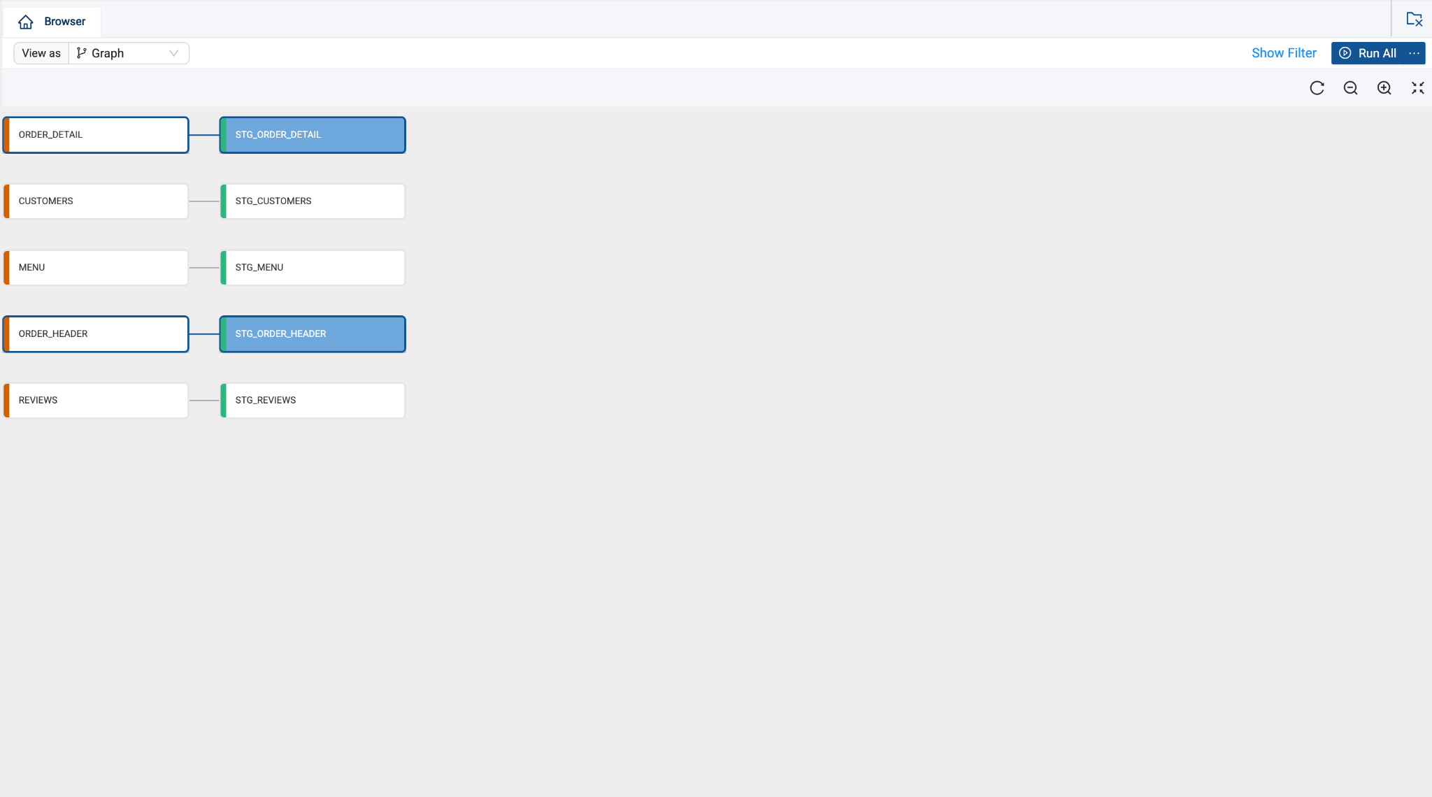
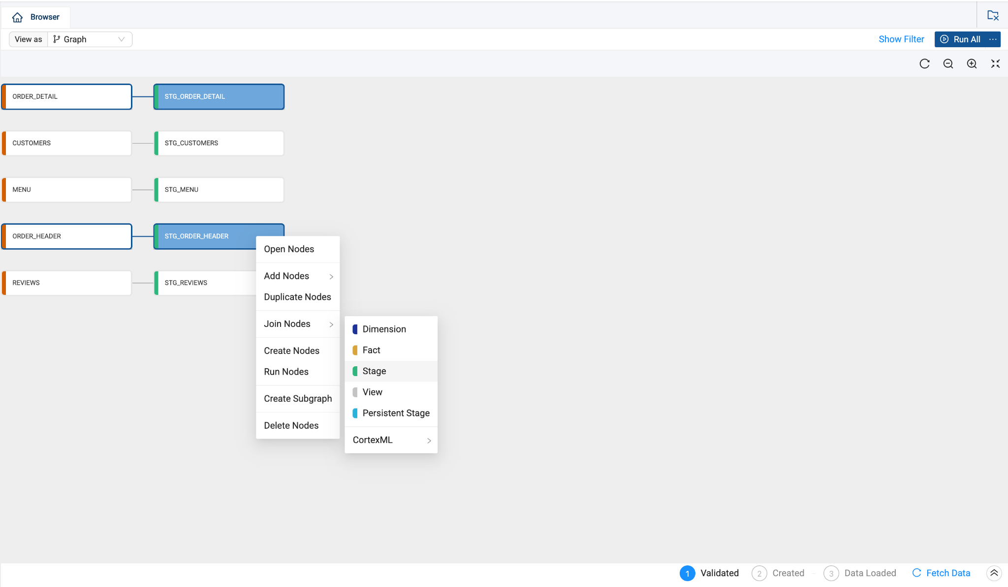
Right click on either node and select Join Nodes, and then select Stage. This will bring you to the node editor of your new Stage node.
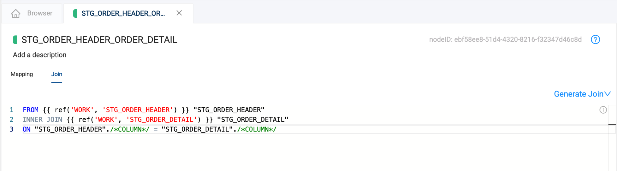
Select the Join tab in the Node Editor. This is where you can define the logic to join data from multiple nodes, with the help of a generated Join statement.

Add column relationships in the last line of the existing Join statement using the code below:

   FROM {{ ref('WORK', 'STG_ORDER_HEADER') }} "STG_ORDER_HEADER"
   INNER JOIN {{ ref('WORK', 'STG_ORDER_DETAIL') }} "STG_ORDER_DETAIL"
   ON "STG_ORDER_HEADER"."ORDER_ID" = "STG_ORDER_DETAIL"."ORDER_ID"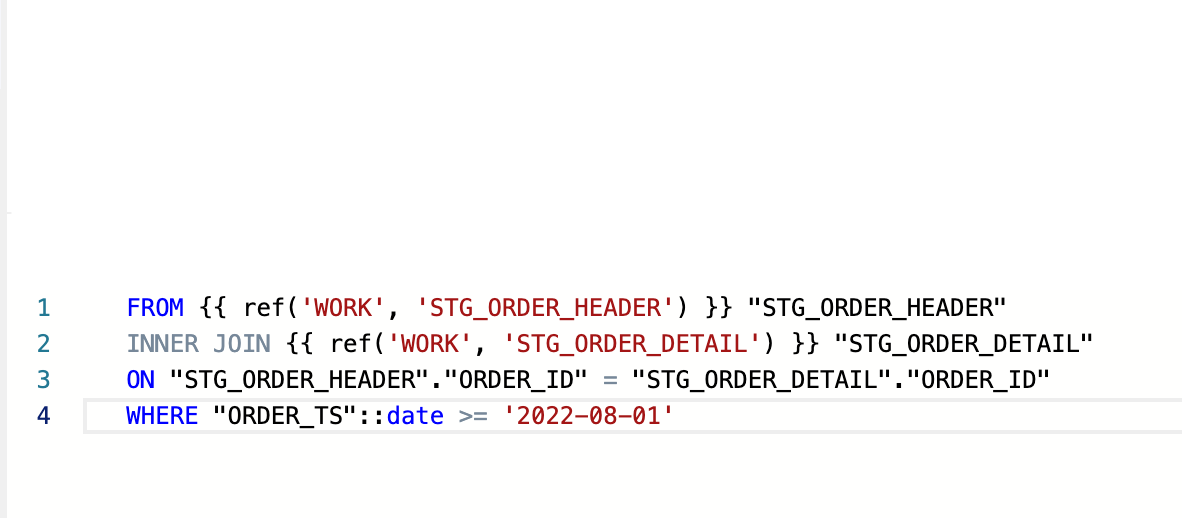

Since both nodes contain a ORDER_ID and DISCOUNT_ID columns, we will need to rename or remove one of the columns to avoid getting a duplicate column name error. Let’s delete the ORDER_ID and DISCOUNT_ID from the STG_ORDER_DETAIL.
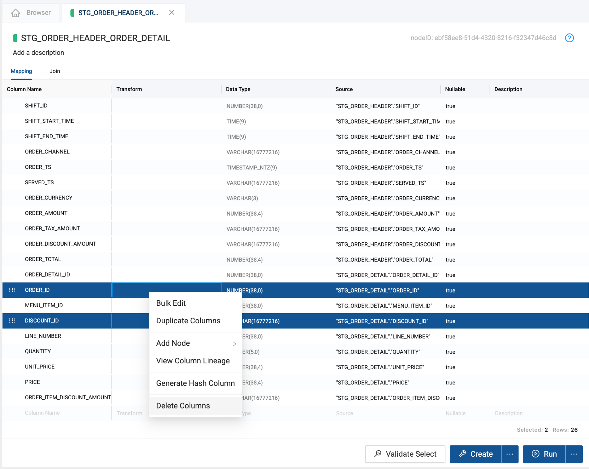
You can rename the node by clicking on the pencil icon next to the node name and give the node a name of your choice. Rename the node to STG_ORDER_MASTER.
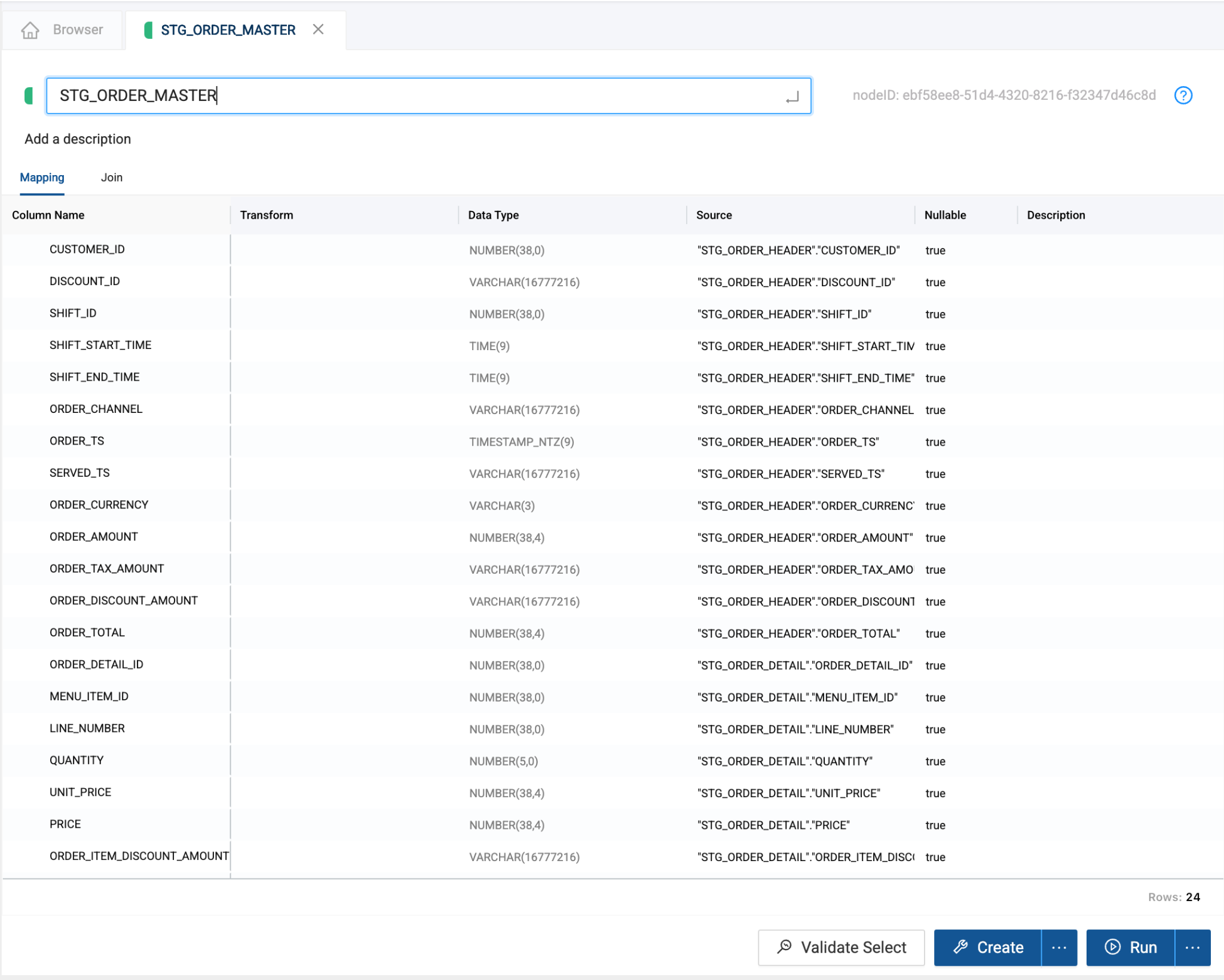
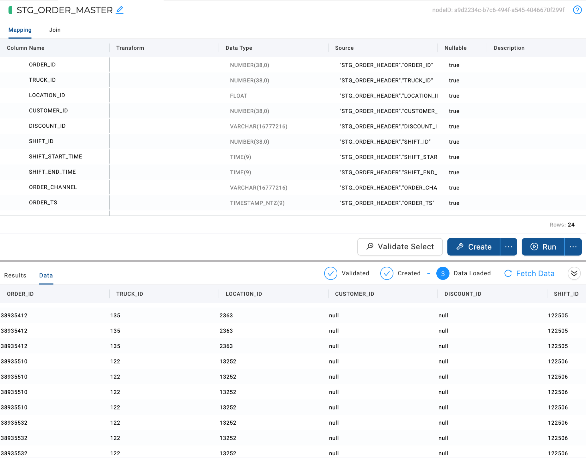
To create your Stage Node, click the Create button in the lower half of the screen. Then click the Run button to populate your STG_ORDER_MASTER node and preview the contents of your node by clicking Fetch Data.

Creating Dimension Nodes

Now let’s experiment with creating Dimension nodes. These nodes are generally descriptive in nature and can be used to track particular aspects of data over time (such as time or location). Coalesce currently supports Type 1 and Type 2 slowly changing dimensions, which we will explore in this section.

Select STG_CUSTOMER and right click, create Dimension node. Because the demographics of your customer base changes over time, creating a Dimension node on top of this data will allow you to capture customer changes over time.
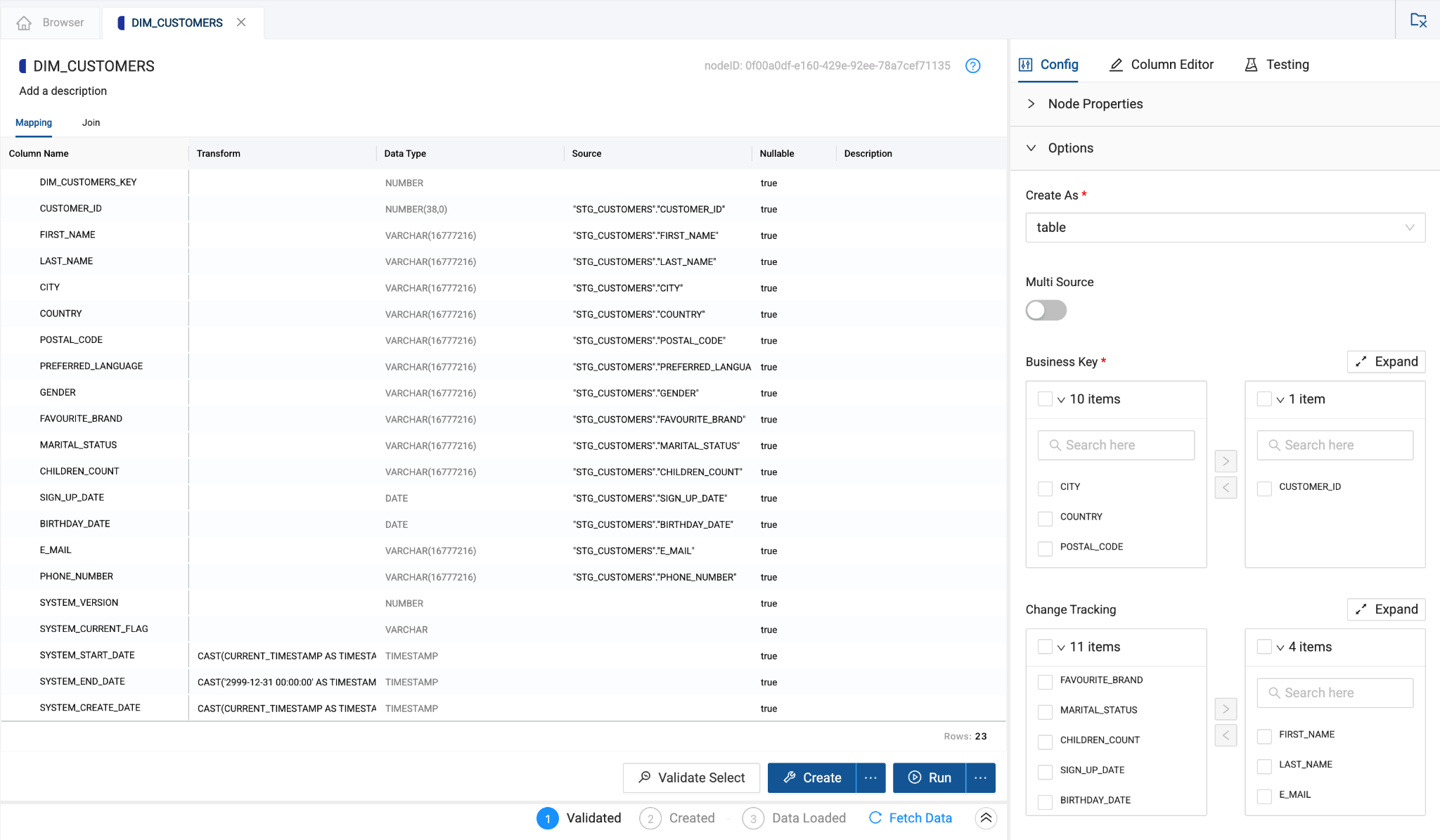
Within the Option configuration section, under Business Key, check the box next to CUSTOMER_ID and press the > button to select it as your business key.
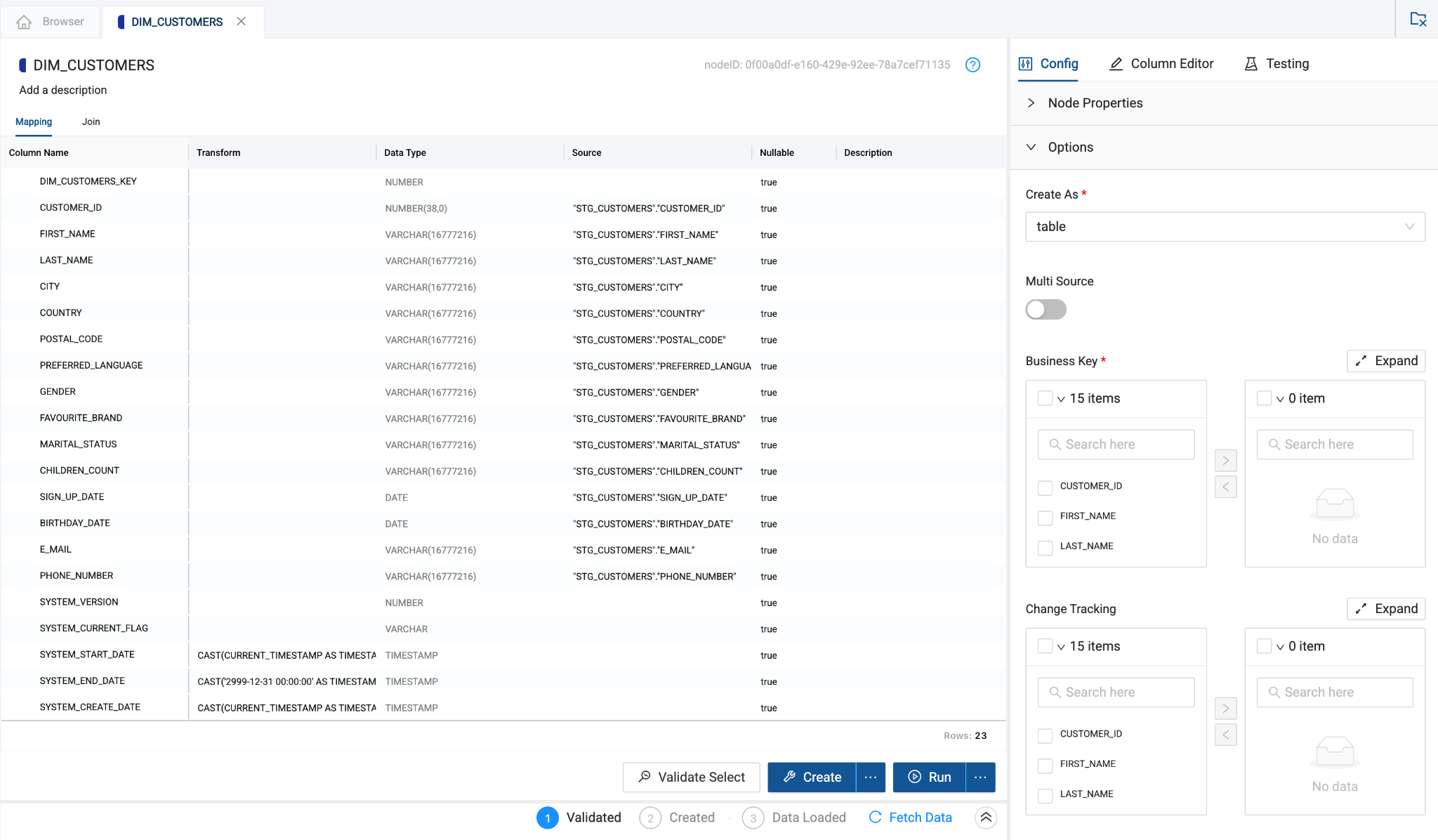
To create a Type 2 dimension, select the FIRST_NAME, LAST_NAME, EMAIL, PHONE_NUMBER columns under Change Tracking. This will allow you to track changes to these columns over time.
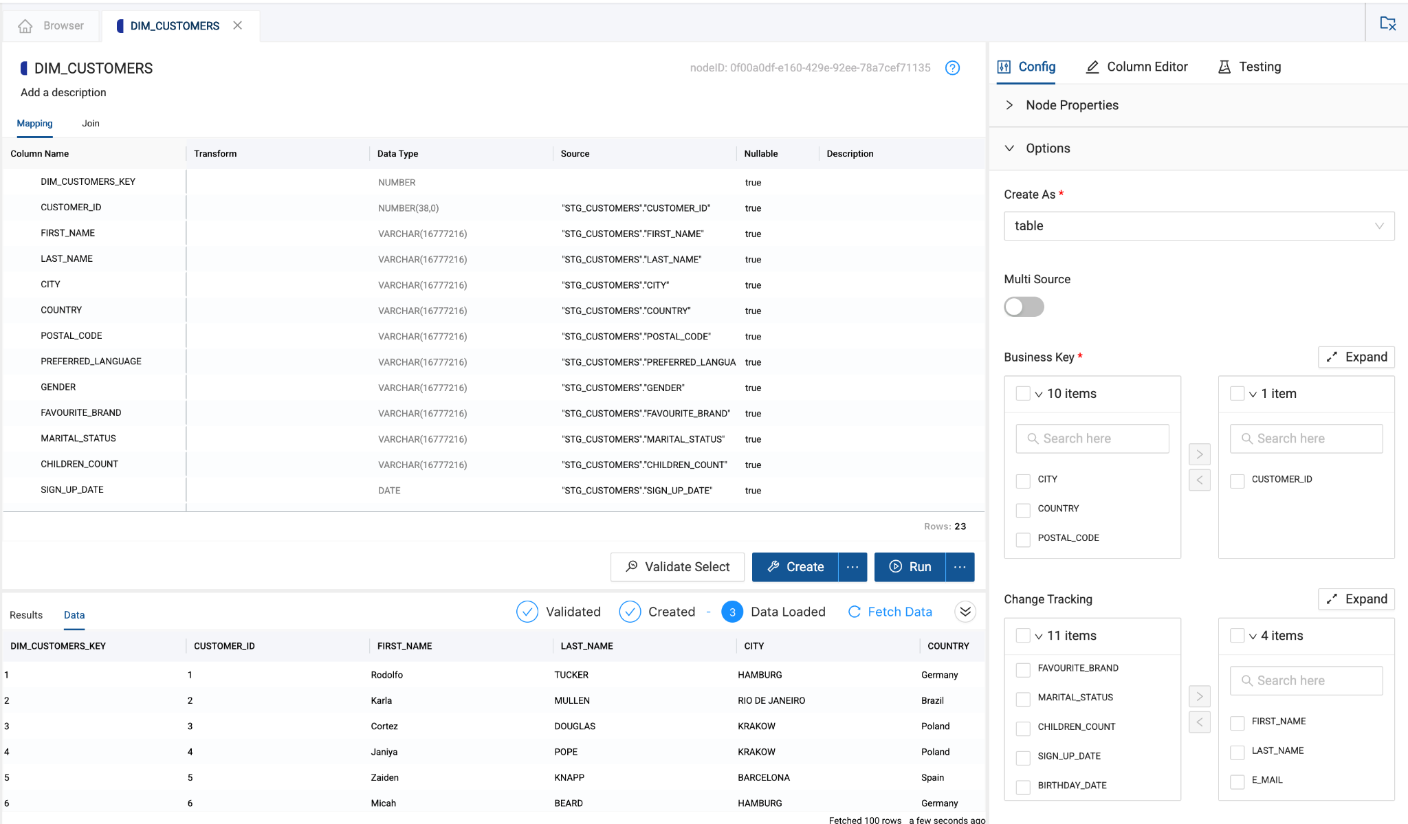
In the lower right of your screen, click the Create button to create your Dimension node and then the Run button to populate it with data.
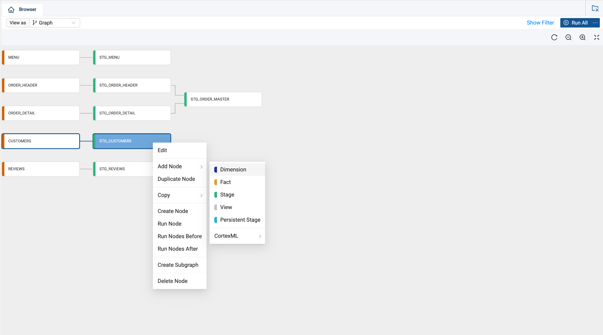
Now let’s create a Type 1 dimension which will help you focus on particular customer details. Navigate back to the Browser tab and select your STG_MENU node. Right click and select Add Node > Dimension from the dropdown menu.
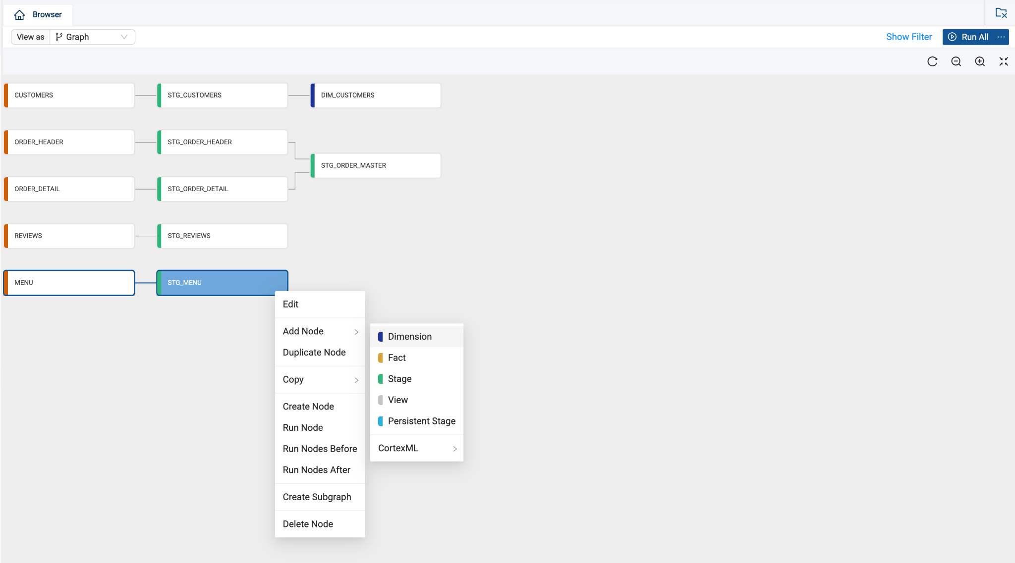
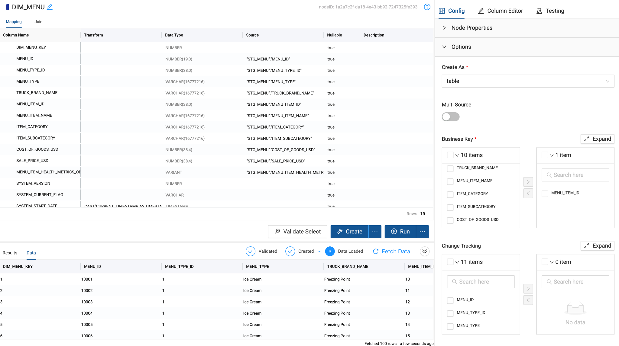
In your DIM_MENU node, navigate to the right and expand the Options drop down in the Config section. Under Business Key, check the box next to MENU_ITEM_ID and press the > button to select it as your business key.
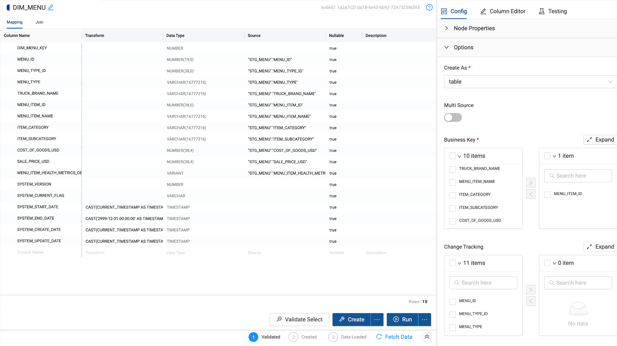
In the lower right of your screen, click the Create button to create your Dimension node and then the Run button to populate it with data.

Creating A Fact Node

Fact nodes represent Coalesce's implementation of a Kimball Fact Table, which consists of the measurements, metrics, or facts of a business process and is typically located at the center of a star or Snowflake schema surrounded by dimension tables.

Let’s create a Fact table to allow us to query the metrics surrounding our customer orders.

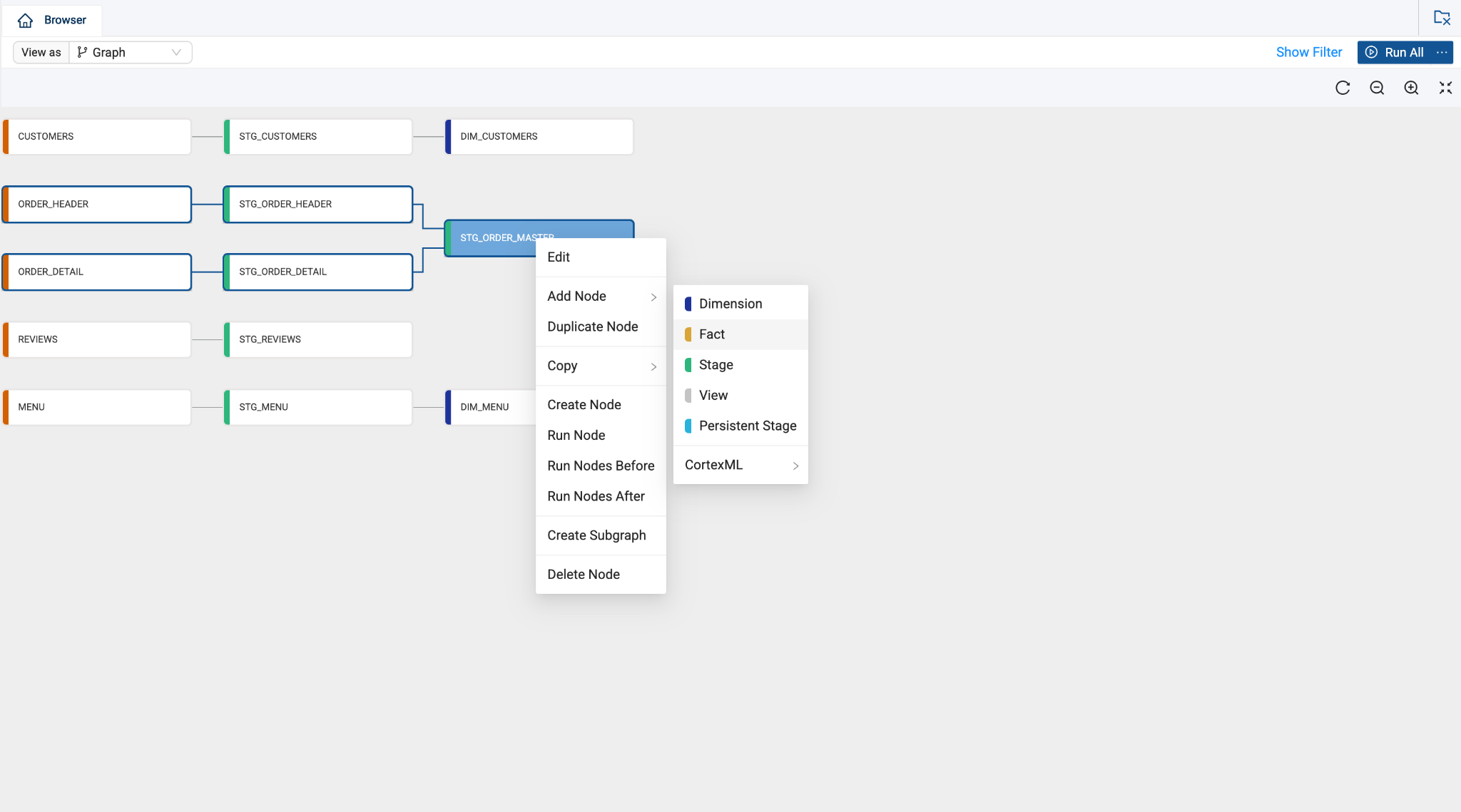
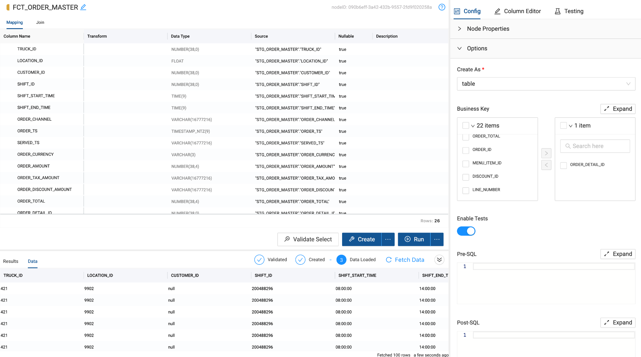
In your Browser tab, select the STG_ORDER_MASTER node. Then right click and select Add Node > Fact.
Navigate to the right and expand the Options drop down in the Config section. Under Business Key, check the boxes next to ORDER_DETAIL_ID. Then press the > button to select them as your business key.
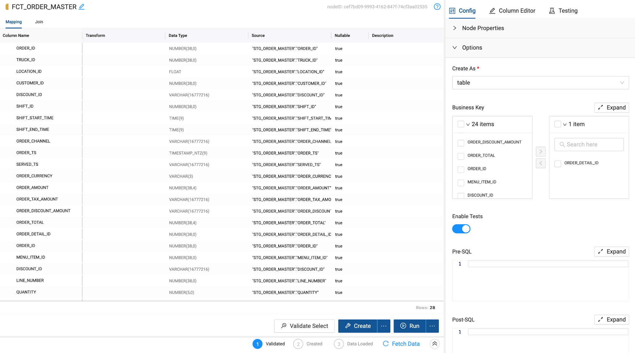
Click the Create and Run buttons to run and populate your FCT_ORDER_MASTER node.

Using Cortex Nodes for Processing Data

Now that we have our fact and dimension nodes, we are going to process the data from the STG_REVIEWS table, allowing us to create a sentiment score for the reviews from each of our customers.

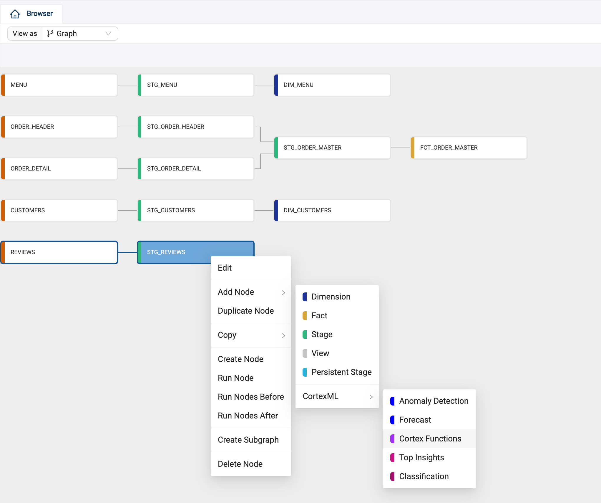
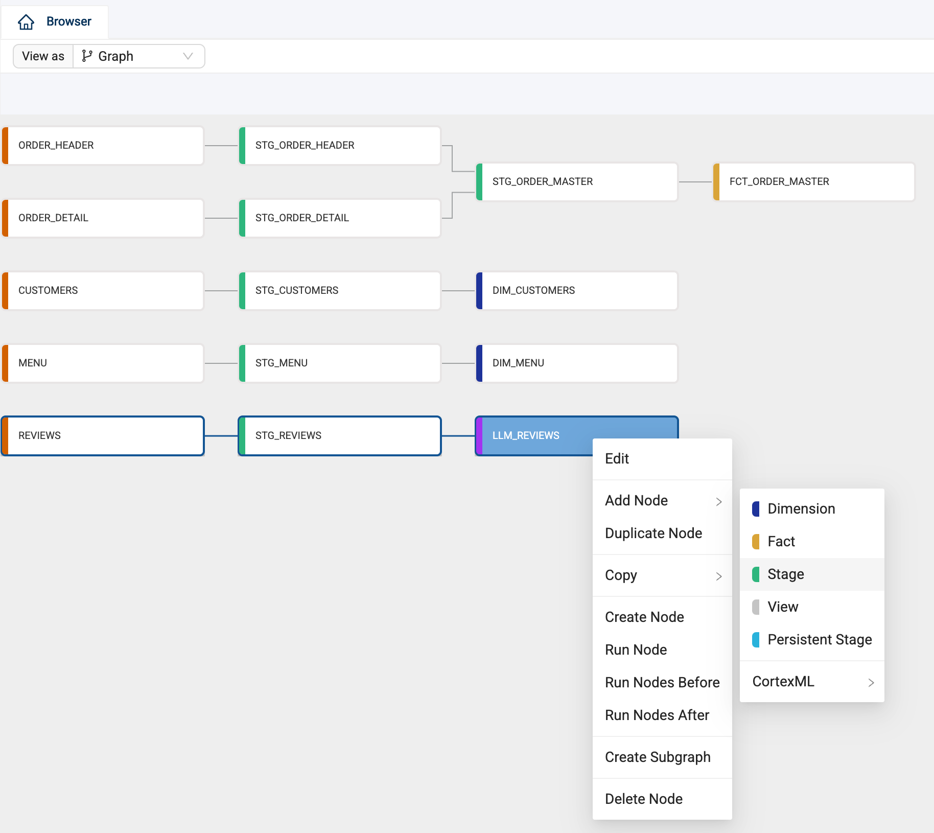
Right click on the STG_REVIEWS and select Add Node -> CortexML -> Cortex Functions.
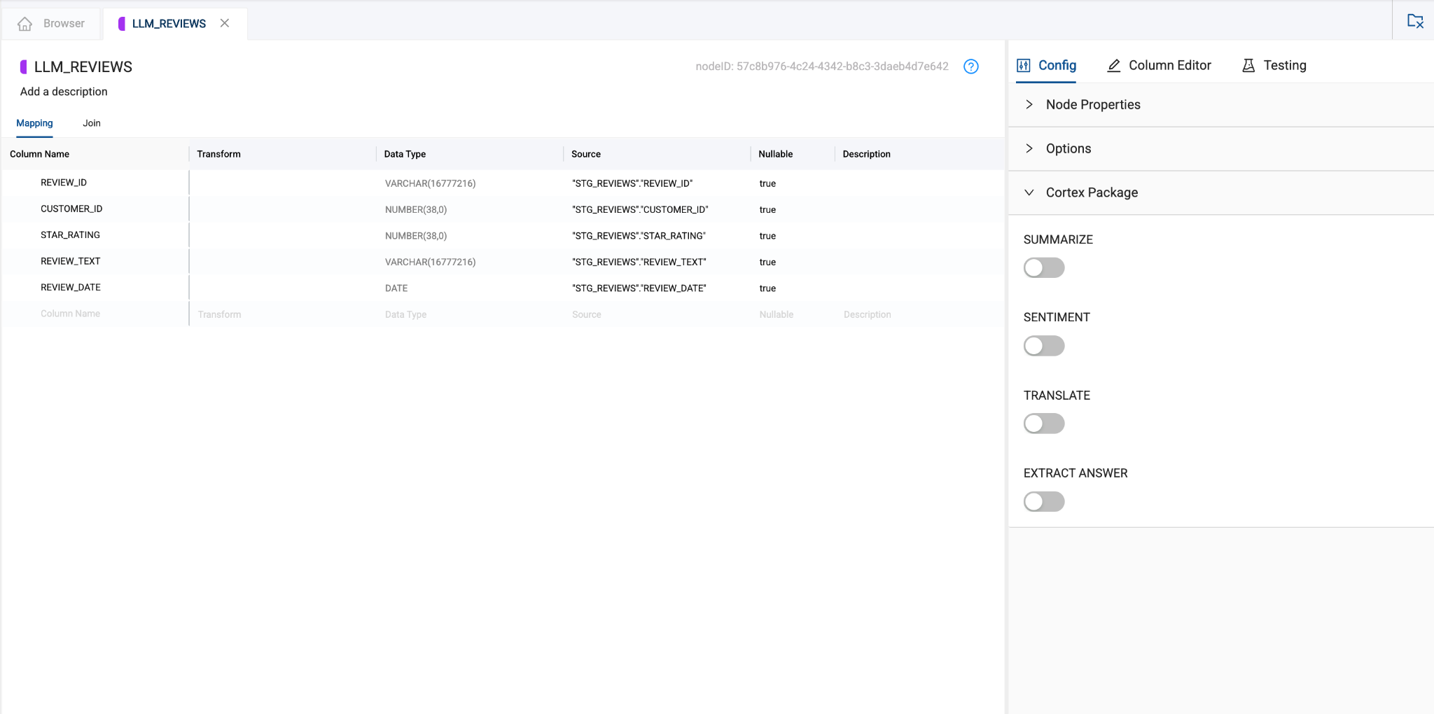
Within the LLM_REVIEWS node, open the Cortex Package dropdown in the Config settings of the node.
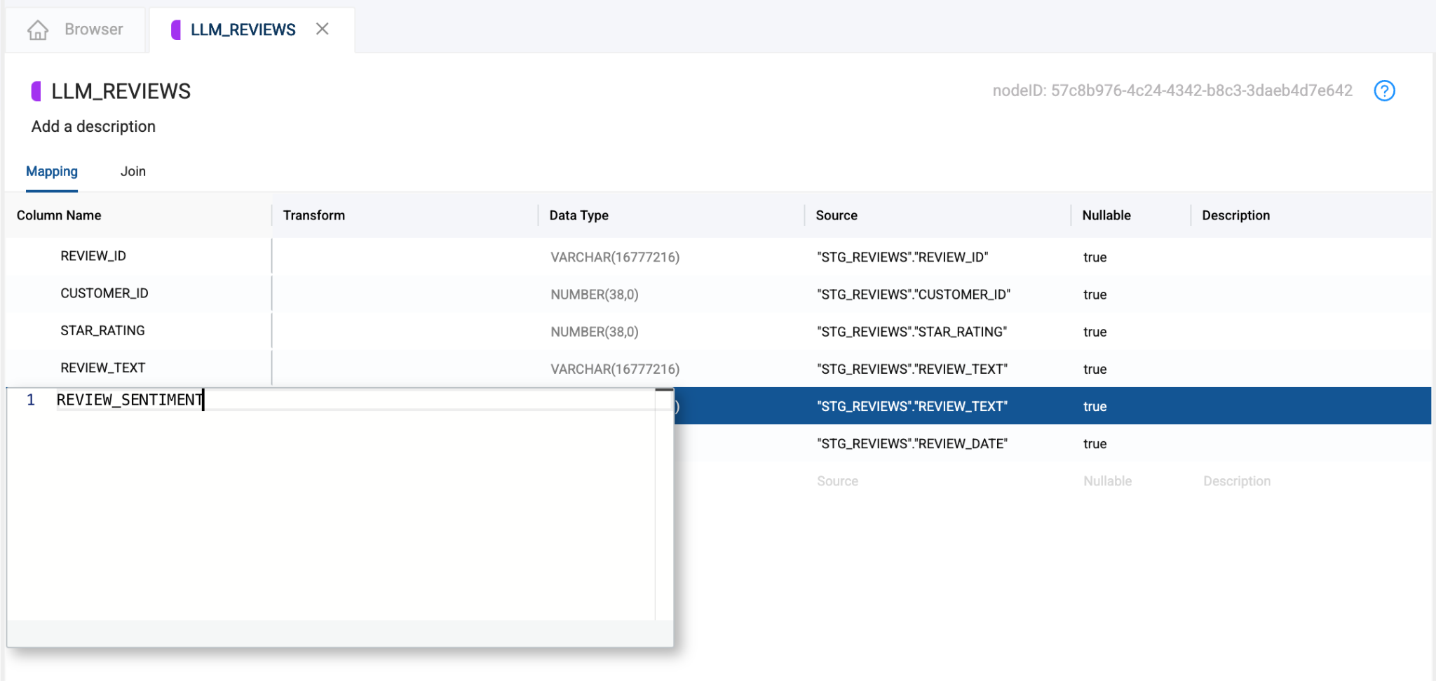
We are going to create a sentiment score based on the reviews left by our customers. These reviews are found in the REVIEW_TEXT column. Duplicate the REVIEW_TEXT column to keep the original text, as the sentiment score we will create, will be in a new column.
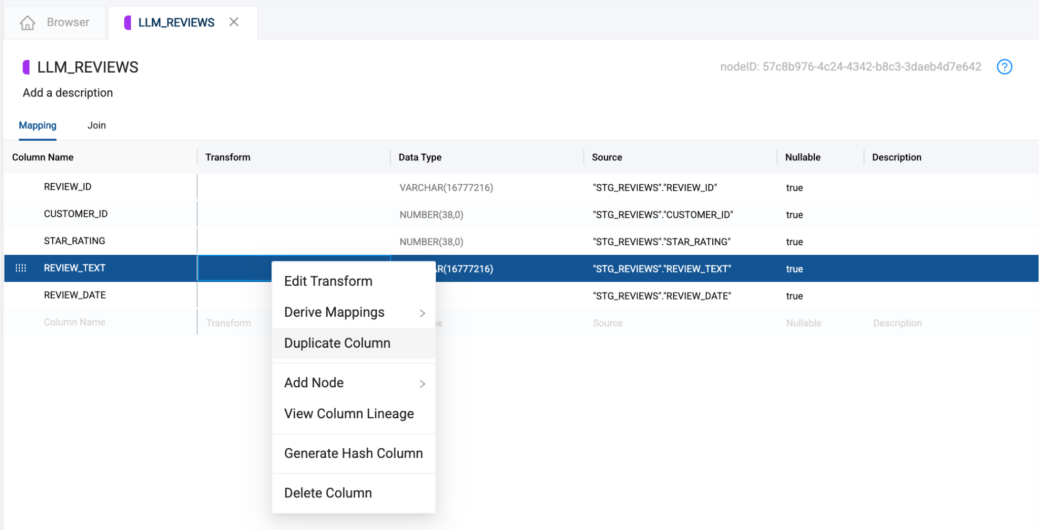
Call the new column REVIEW_SENTIMENT. You can do this by double clicking on the new column name.
Select the Sentiment toggle on the right side of the node in the Cortex Package configuration options. Then, select the REVIEW_SENTIMENT column we just created.
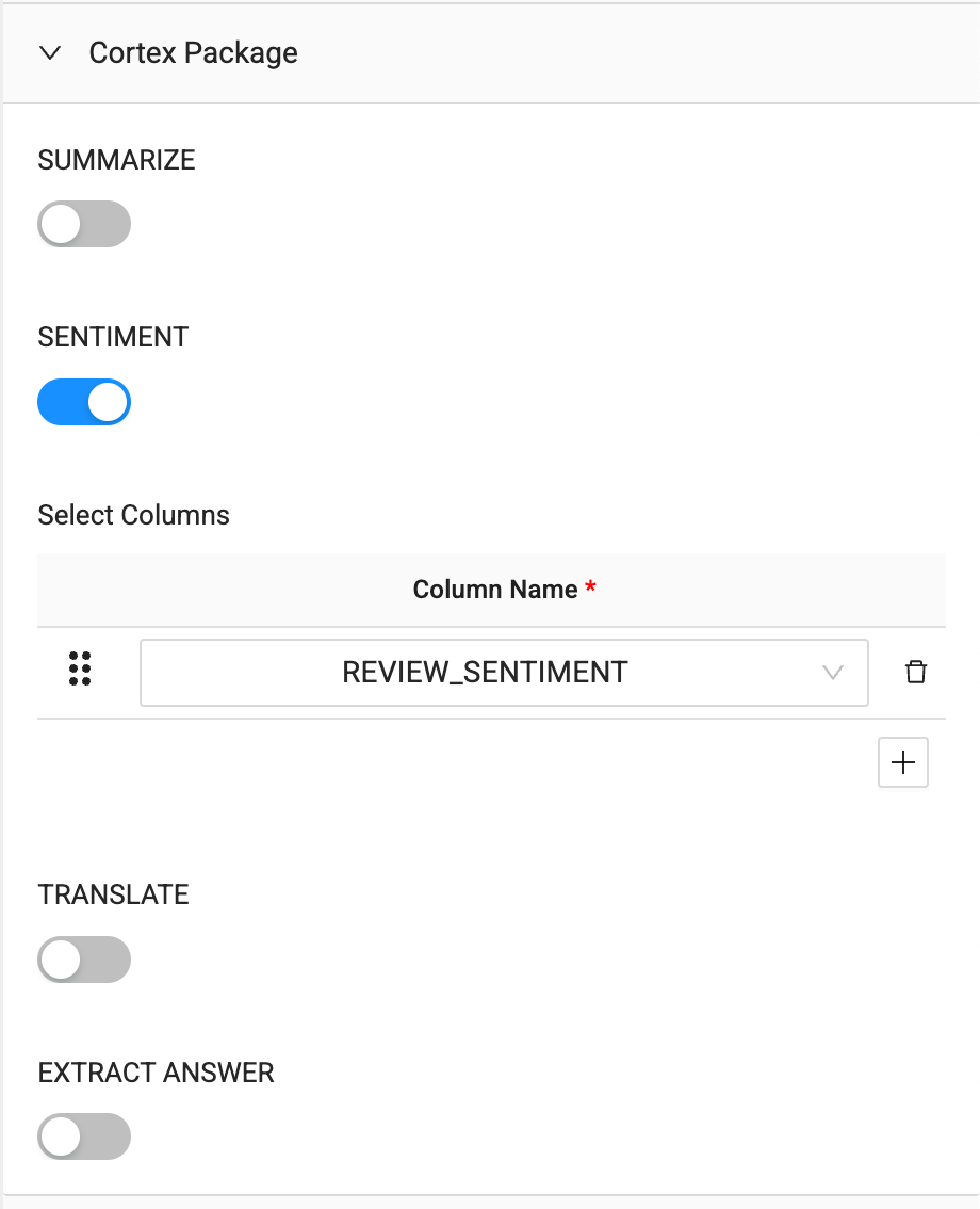
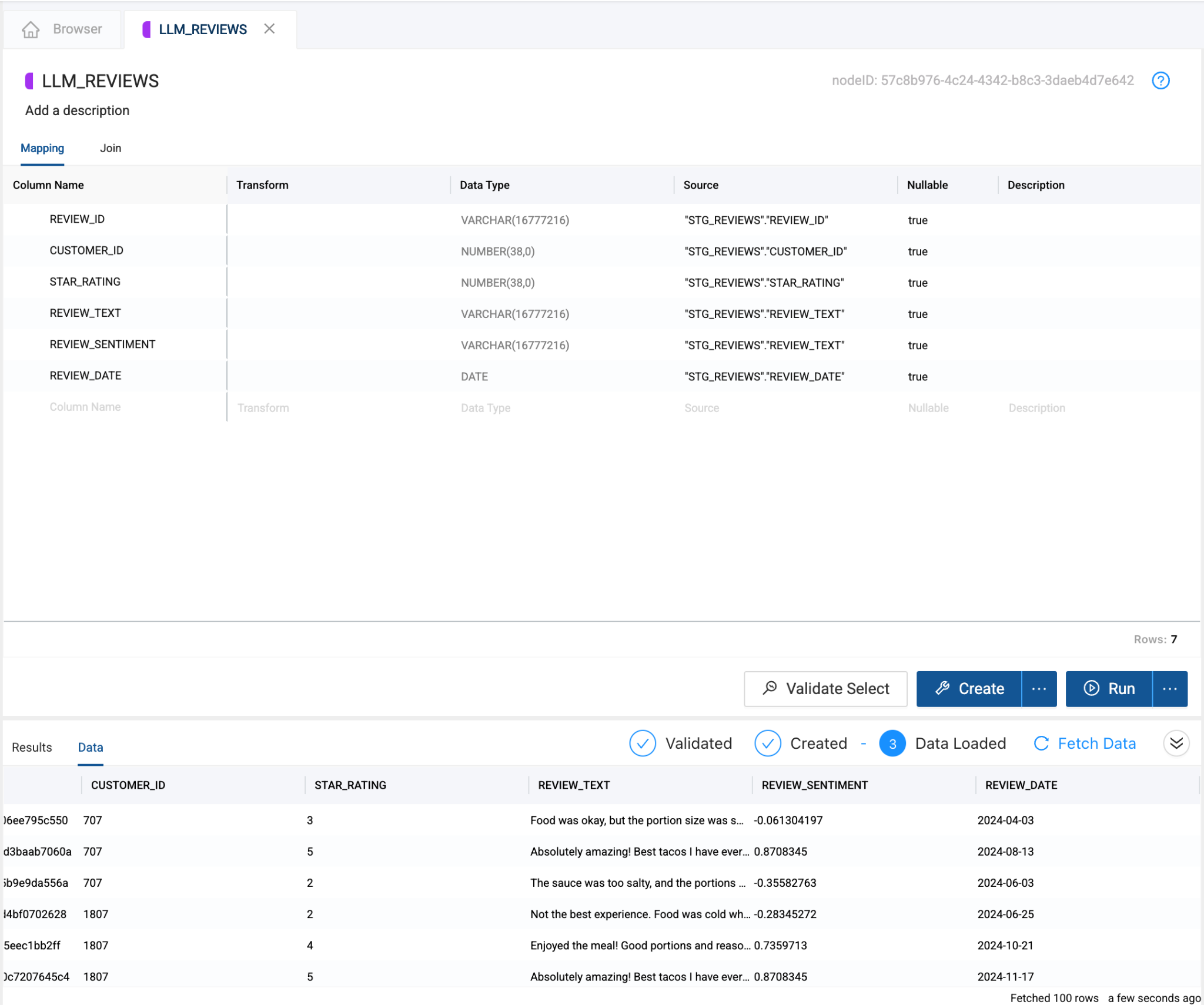
And that’s it. Coalesce will handle the rest. Select Create and Run to create the object and populate it with data, which will include the sentiment score.
Next, we’ll process this data a bit more, so we can see the average review and sentiment for our customers. Right click on the LLM_REIVEWS node and select Add Node -> Stage.
Rename the node to STG_CUSTOMER_SENTIMENT.
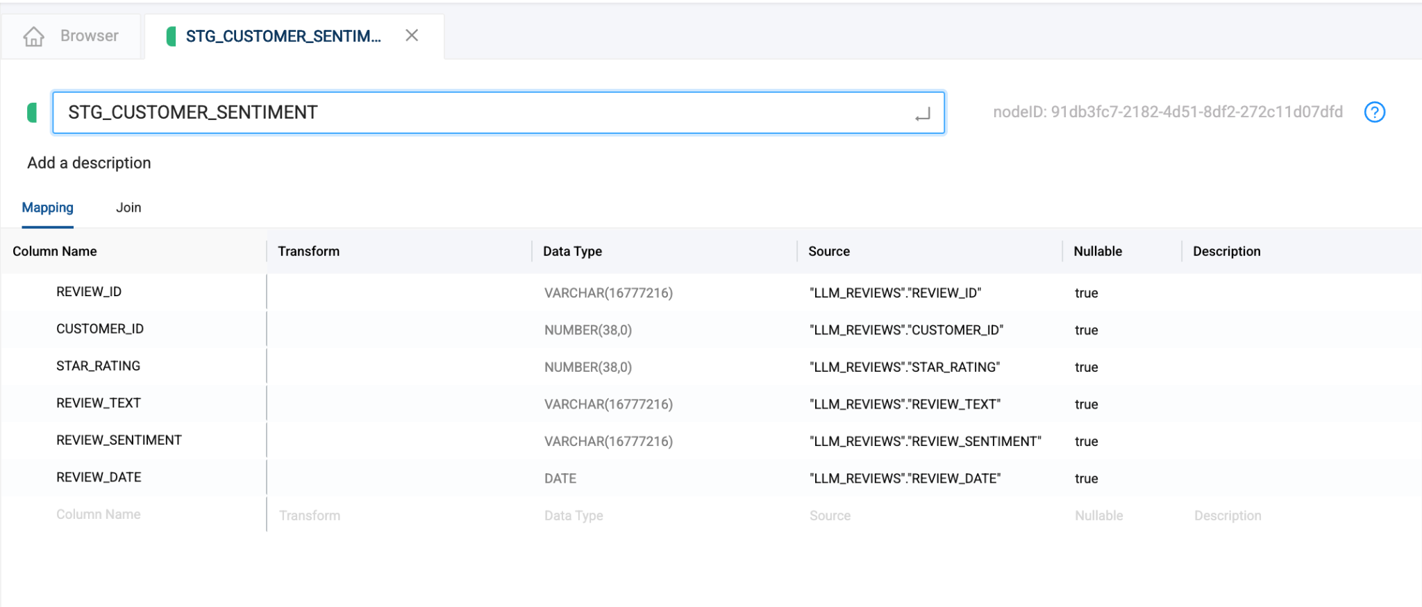
Next, remove the following columns from the node:
- REVIEW_ID
- REVIEW_TEXT
- REVIEW_DATE
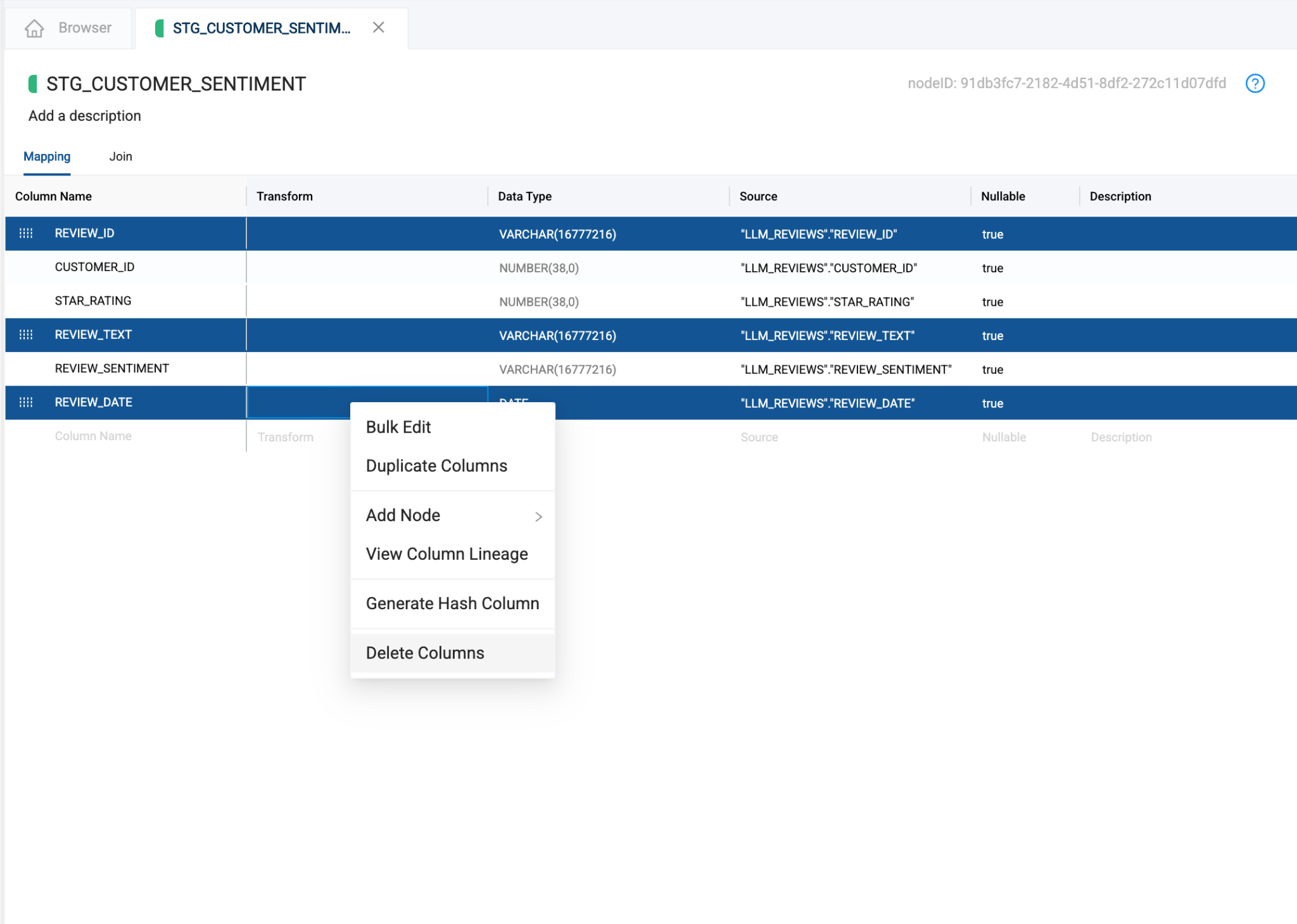
We want to know the average sentiment and star rating for each of our customers, as many of our customers have left multiple reviews. We can use the Coalesce bulk editing transformation functionality for this. Select the STAR_RATING and REVIEW_SENTIMENT columns and right click on either one and select Bulk Edit.
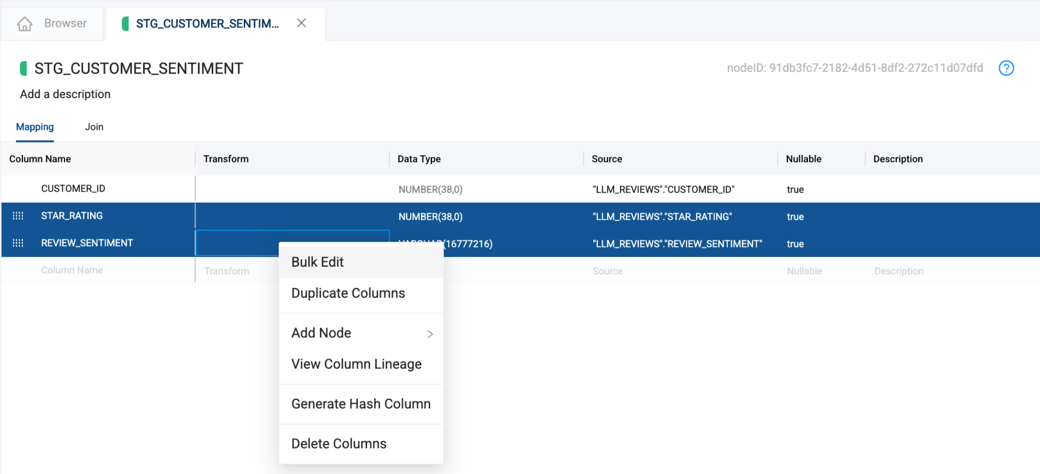
In the attributions section, select Transform, as this is the operation we want to apply in bulk.
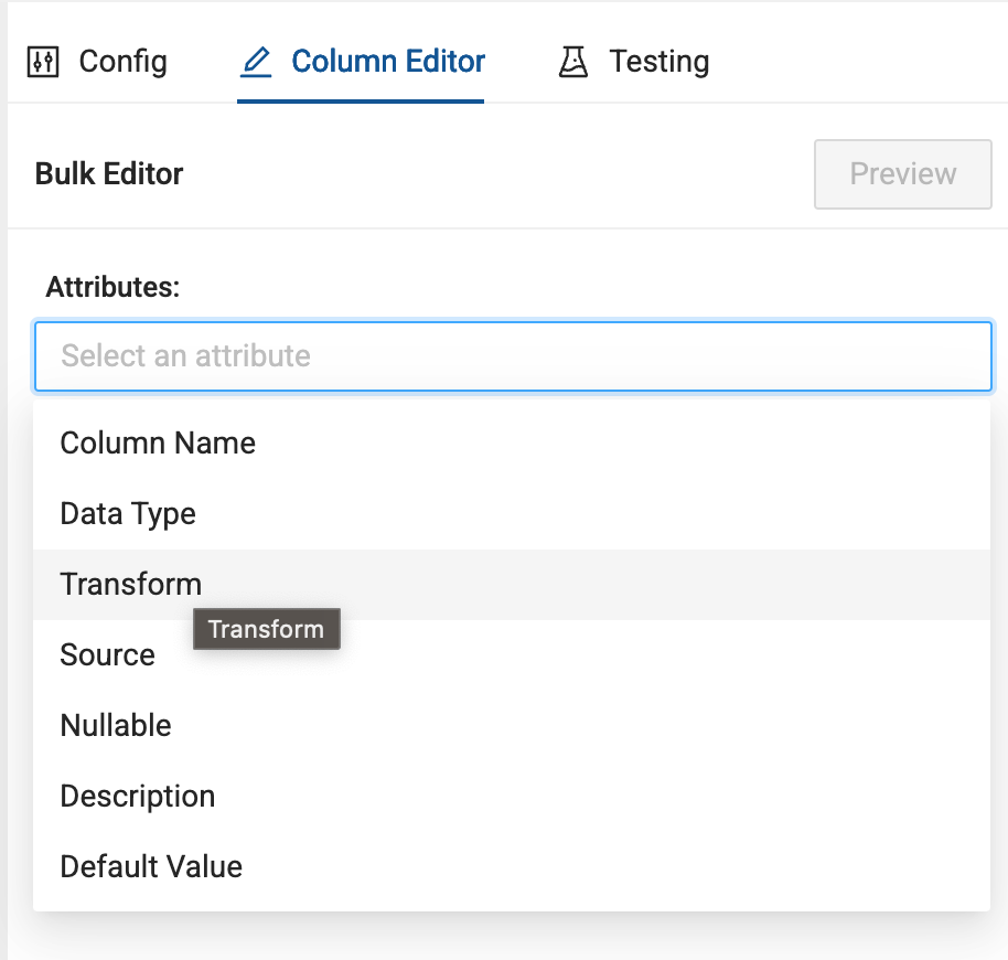
In the transform SQL editor, copy and paste the following snippet of code.
```
AVG({{SRC}})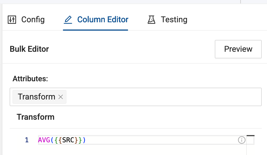
```
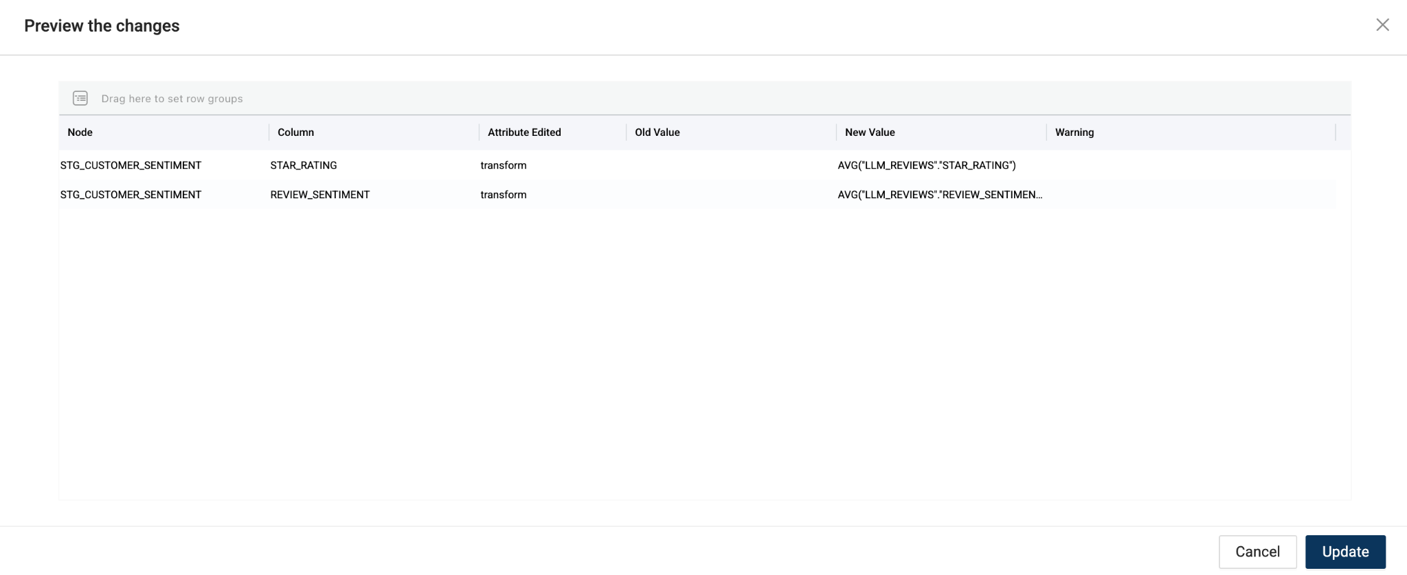
Select the Preview button to view the changes and then select Update to apply the changes to your node.
Finally, since we are using aggregate functions in SQL, we need to use a GROUP BY for our non-aggregated column. In the Join SQL Editor, start a new line and supply the following SQL: GROUP BY ALL
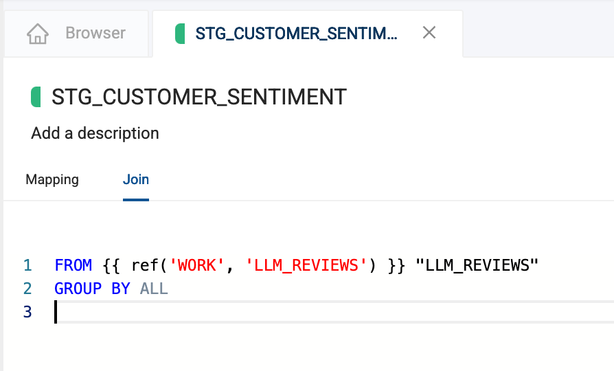
Now Create and Run the node.
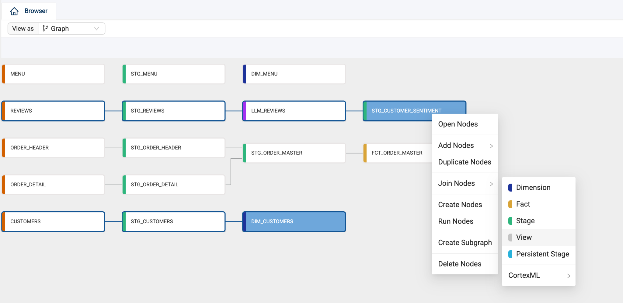
Navigate back to the Browser and now we can join the DIM_CUSTOMER node to the STG_CUSTOMER_SENTIMENT node we just created. Select both nodes and right click on either node and select Join Nodes -> View.
Rename the node to V_CUSTOMER.

Navigate to the Join table to configure the join. In this case, we need to join on CUSTOMER_ID. Use the code below to configure the join:

FROM {{ ref('WORK', 'STG_CUSTOMER_SENTIMENT') }} "STG_CUSTOMER_SENTIMENT"

LEFT JOIN {{ ref('WORK', 'DIM_CUSTOMERS') }} "DIM_CUSTOMERS"

ON "STG_CUSTOMER_SENTIMENT"."CUSTOMER_ID" = "DIM_CUSTOMERS"."CUSTOMER_ID"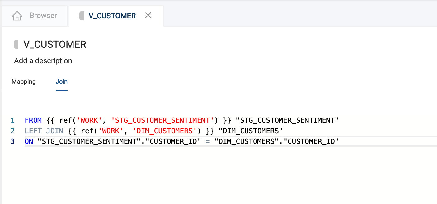

Back in the mapping grid, remove one of the CUSTOMER_ID columns, as the table can’t contain two of the same named column.
Select Create when ready to create your view. Congratulations. You now have a view that users can query to learn about the sentiment of your customers.

Creating ML Processing Node

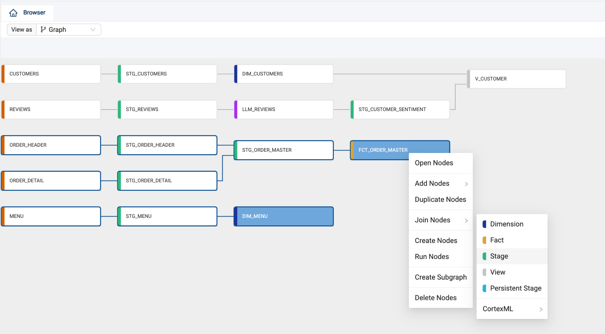
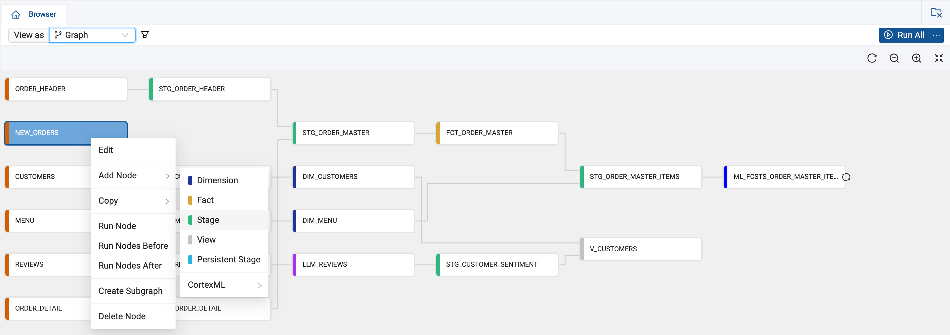
To finish preparing your data for ML forecasting, we’ll perform one more join. Navigate back to the Browser and select the FCT_ORDER_MASTER node and the DIM_MENU node by holding down the shift key and clicking on both nodes. Right click on either node and select Join Nodes, and then select Stage. This will bring you to the node editor of your new Stage node.
Select the Join tab in the Node Editor. This is where you can define the logic to join data from multiple nodes, with the help of a generated Join statement. Add column relationships in the last line of the existing Join statement using the code below:
```
FROM {{ ref('WORK', 'DIM_MENU') }} "DIM_MENU"
INNER JOIN {{ ref('WORK', 'FCT_ORDER_MASTER') }} "FCT_ORDER_MASTER"
ON "DIM_MENU"."MENU_ITEM_ID" = "FCT_ORDER_MASTER"."MENU_ITEM_ID"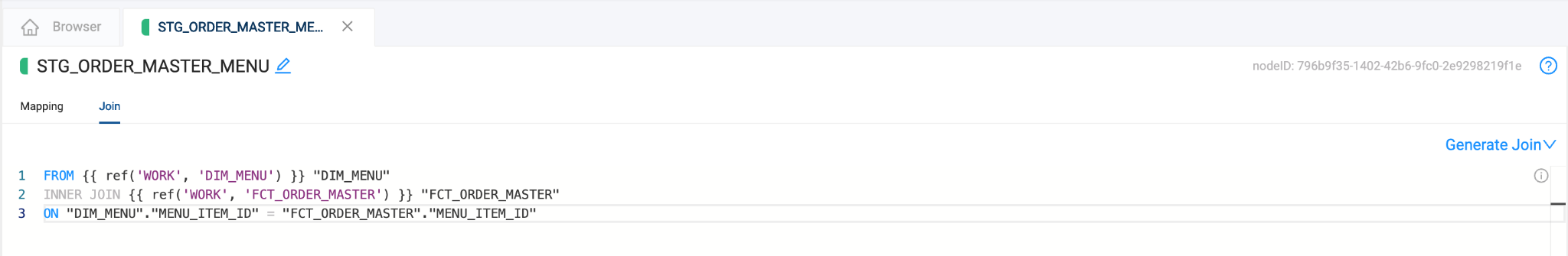
```
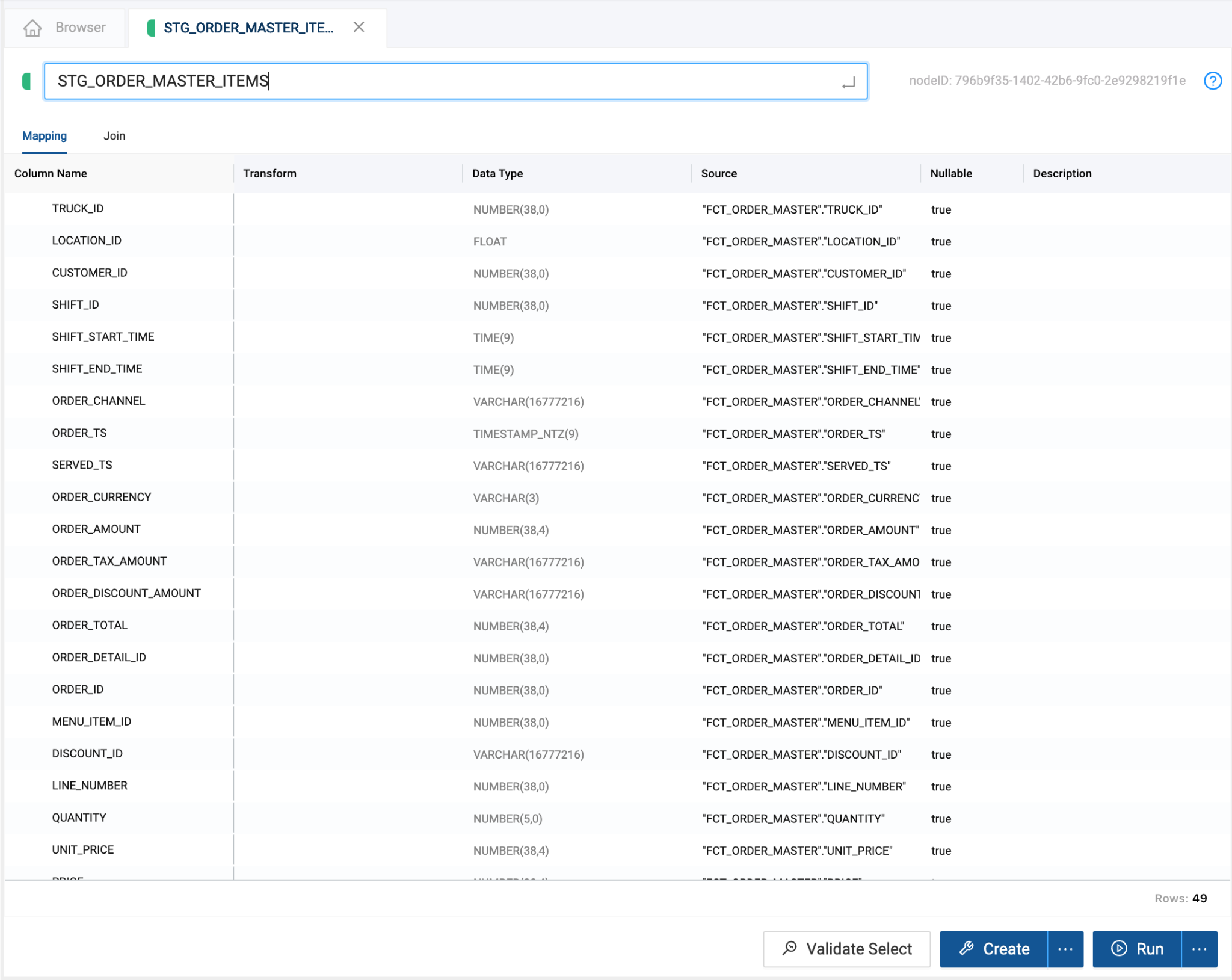
You can rename the node by clicking on the pencil icon next to the node name and give the node a name of your choice. Rename the node STG_ORDER_MASTER_ITEMS.
Back in the mapping grid, delete one of the duplicate MENU_ITEM_ID columns, as well as all the SYSTEM_ columns and then create and run the node.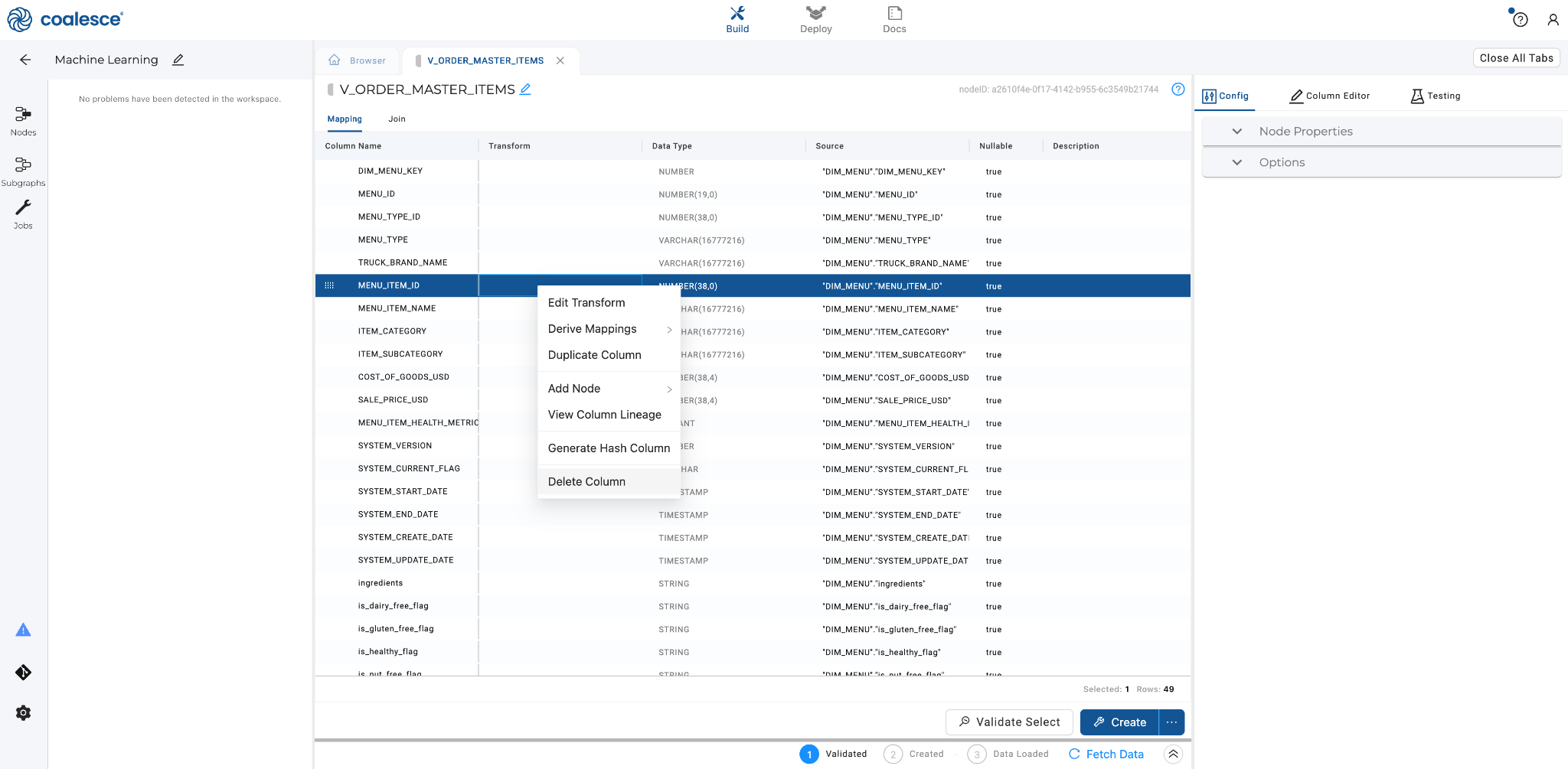

Transforming Data in a Node

Now we will prepare the data for our ML forecast by selecting the columns we want to work with and applying single column transformations to that data.

The ML Forecast node we will use later in the lab will rely on three columns to produce a forecast:

Series column
Timestamp column
Target column

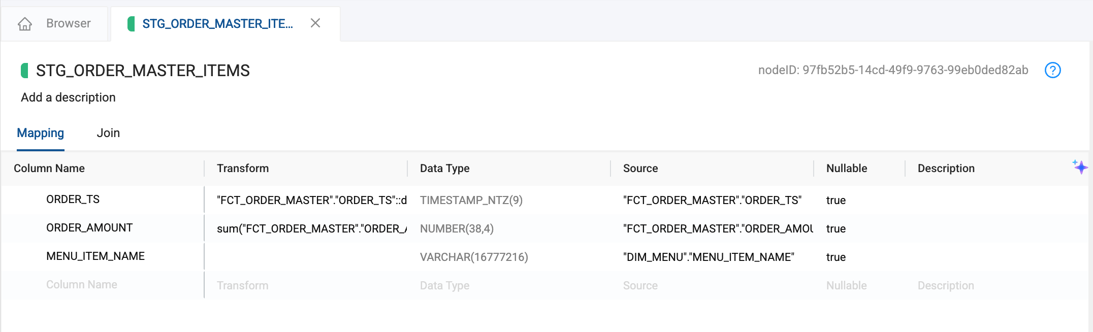
We will structure our STG_ORDER_MASTER_ITEMS node so that it only contains the columns we will need for our ML Forecast Node.

MENU_ITEM_NAME -> Series column
ORDER_AMOUNT -> Target column
ORDER_TS -> Timestamp column

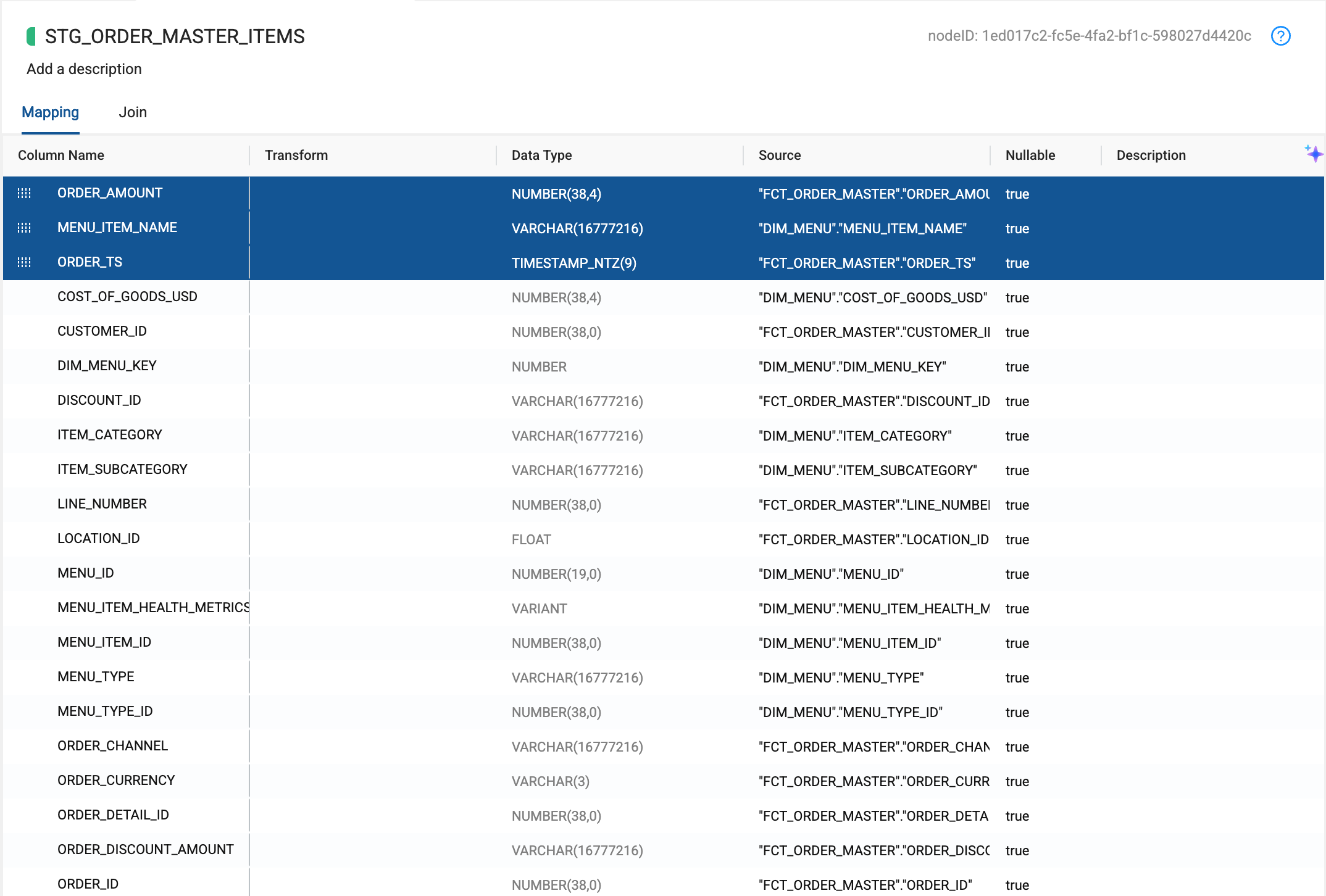
To structure the node with the columns that we need, the first thing we will do is rename the columns we want to keep. Select the ORDER_AMOUNT, ORDER_TS, and MENU_ITEM_NAME columns, and right click on either of the columns and select, Bulk Edit.
In the Bulk Editor, select the Column Name attribute and copy and paste the code below to apply a FORECAST prefix to each of the columns we want to keep. Select Preview -> Update to rename the columns.
```
FORECAST_{{column.name}}
```
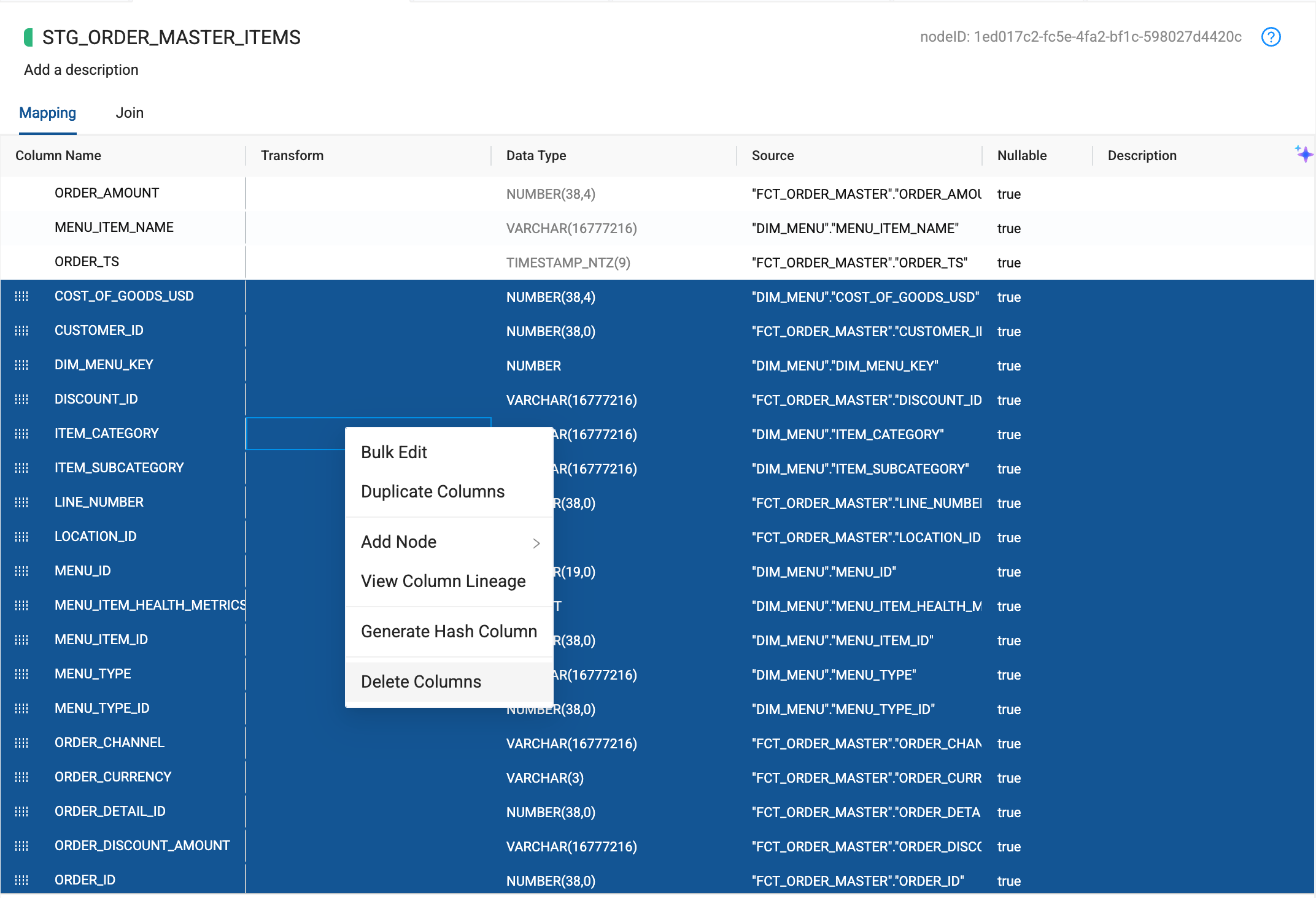
Click on the Column Name column header in the mapping grid to sort the column names in alphabetical order. Using the shift key, select all of the columns that do not contain a FORECAST_ prefix, right click on them, and delete them.
With the columns we need for our forecast in this node, we will now apply some column transformations. Currently the Timestamp column records values down to the second interval. For this lab, we want to predict order values at the day level. Let’s add this transformation. Select the FORECAST_ORDER_TS column and click into the transform field in the mapping grid. You can cast a timestamp as a date, removing the seconds, minutes, and hours, by using the transformation below:
```
{{SRC}}::date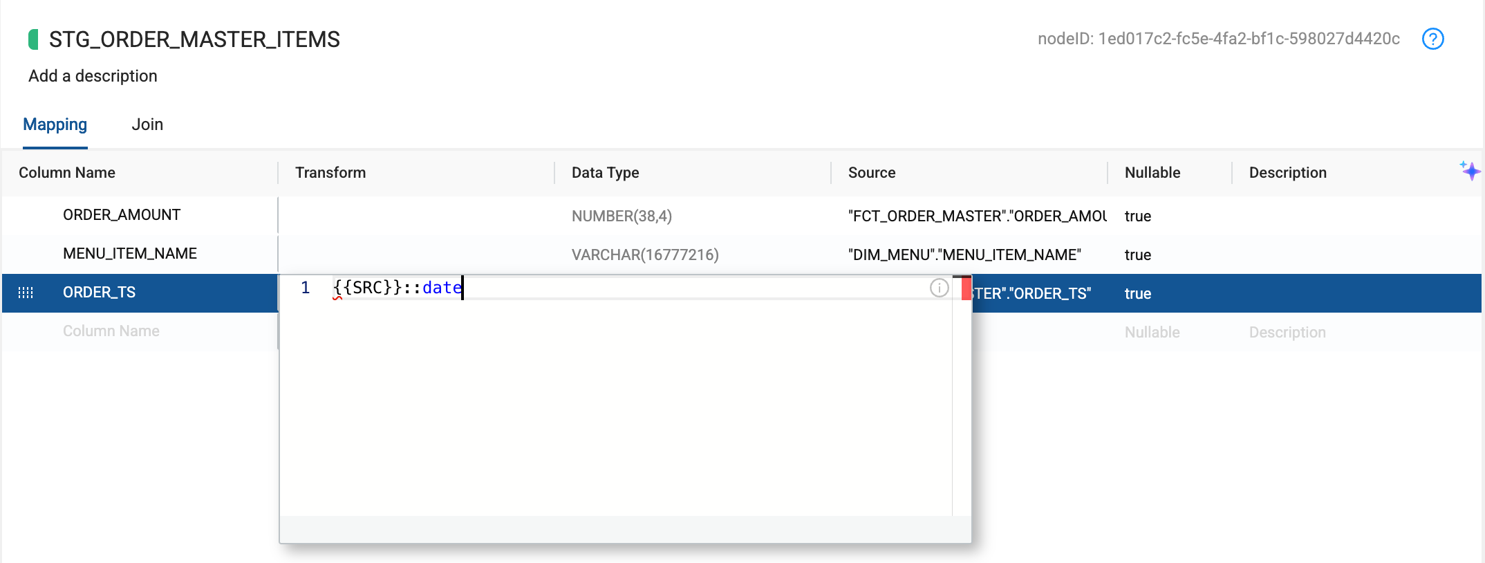
```
Next, we need to aggregate our sales at the day level. We can use a sum function for this. You can use the transformation here to sum the ORDER_AMOUNT column.
```
sum({{SRC}})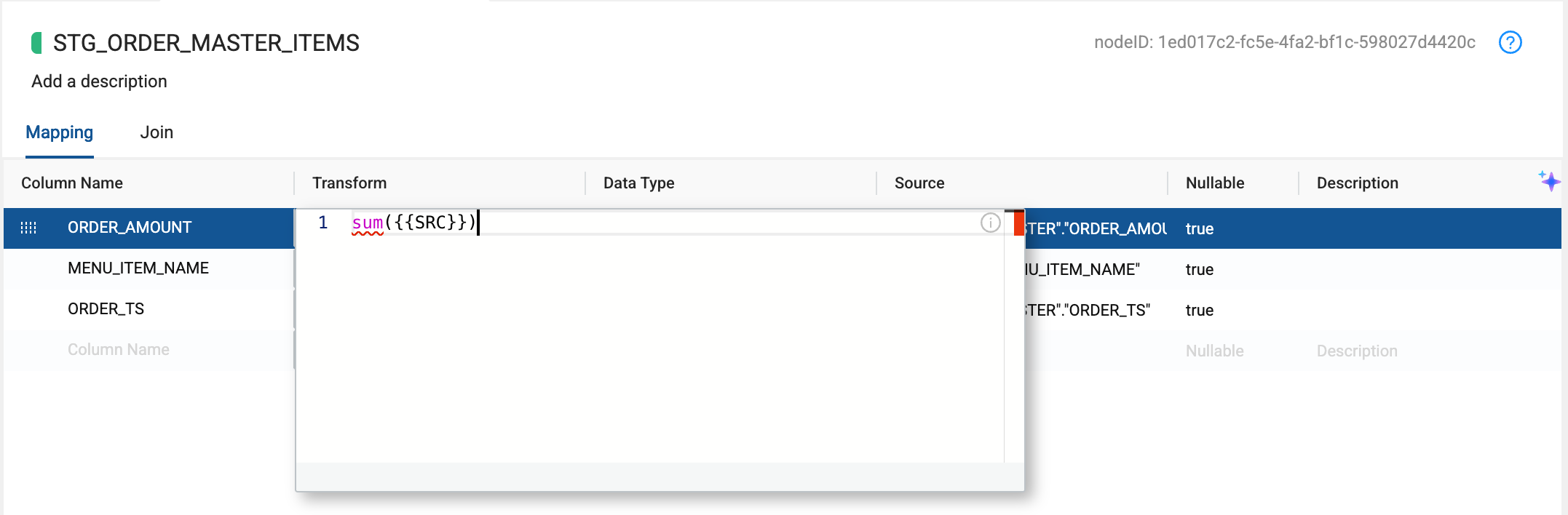
```
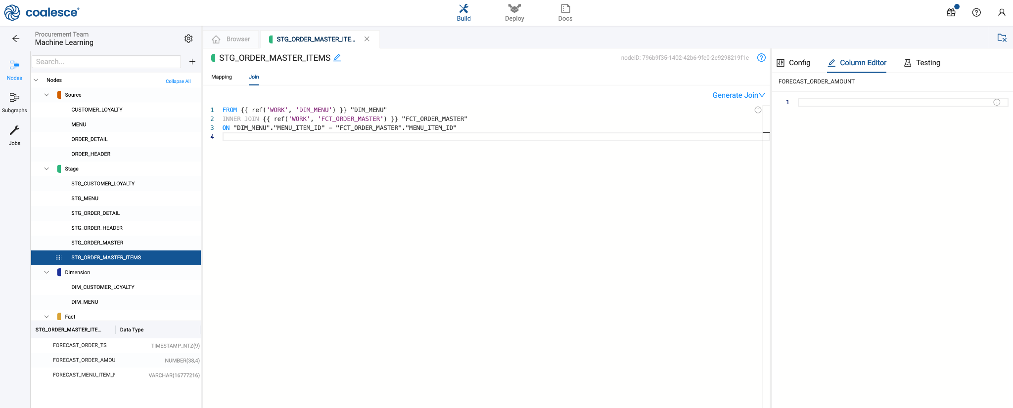
We will leave the MENU_ITEM_NAME column as it is. However, because we have included an aggregate function, we will need to use a GROUP BY in the node. Navigate to the JOIN tab so we can finish preparing this node.
Because we are using an aggregate function, we will add a GROUP BY statement. Additionally, the data set is relatively large, so we will narrow down the items we are working with by providing a filter. Within the Join tab, add a new line in the editor by hitting the enter key. Next, type GROUP BY within the editor, followed by the two non-aggregated columns, MENU_ITEM_NAME and ORDER_TS. You can copy the code for this below:
```
FROM {{ ref('WORK', 'DIM_MENU') }} "DIM_MENU"
INNER JOIN {{ ref('WORK', 'FCT_ORDER_MASTER') }} "FCT_ORDER_MASTER"
ON "DIM_MENU"."MENU_ITEM_ID" = "FCT_ORDER_MASTER"."MENU_ITEM_ID"
WHERE "ITEM_CATEGORY" = 'Beverage' and "FORECAST_ORDER_TS"::date >= '2022-08-01'
GROUP BY ALL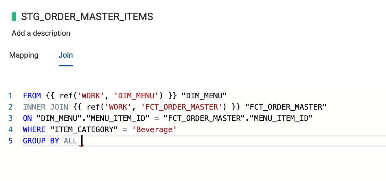
```
Create and Run the node to populate it with data for the next section of the lab guide.

Adding an ML Forecast Node

The next step in building out this data pipeline for getting your ML Forecast Node operational, we will add in the ML Forecast Node to the pipeline.

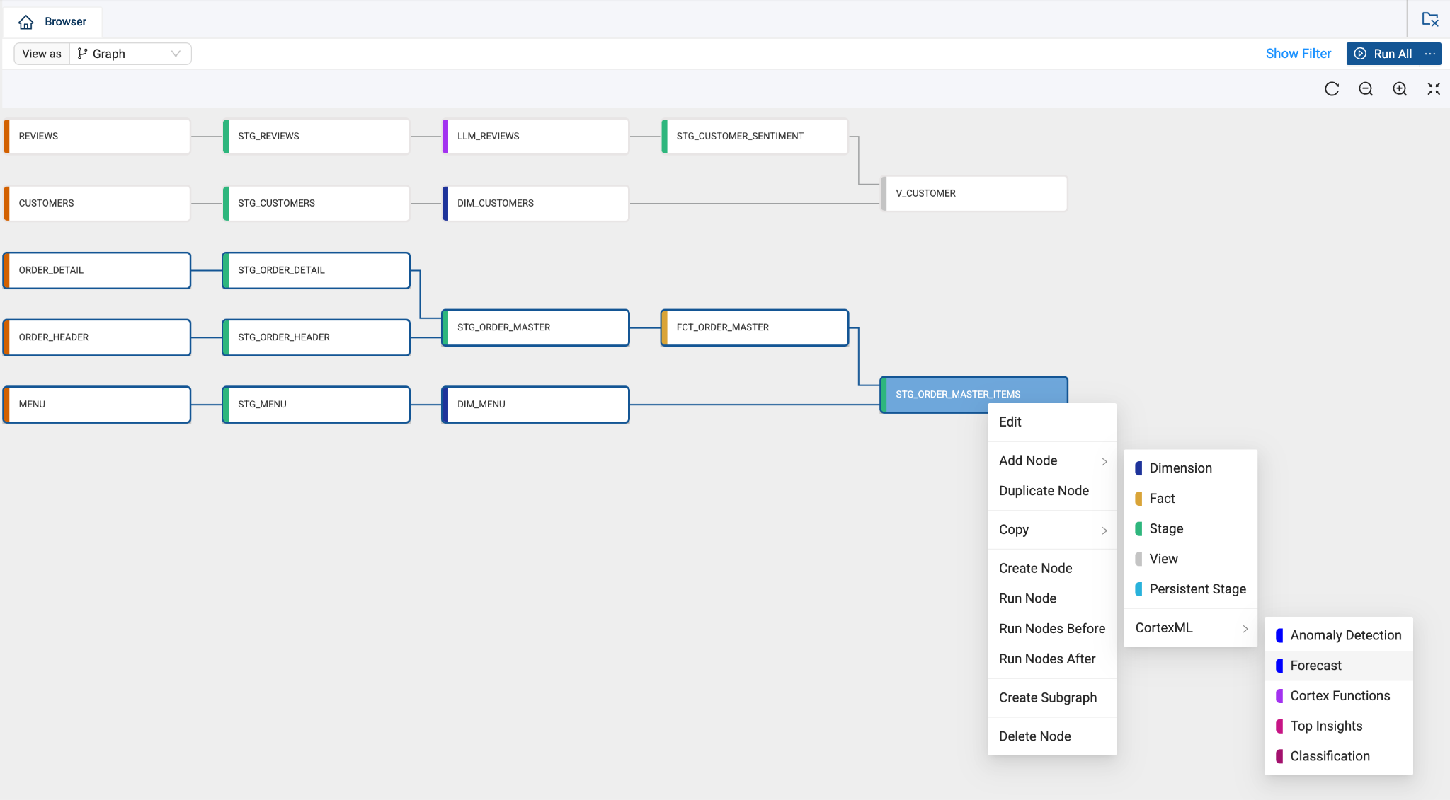
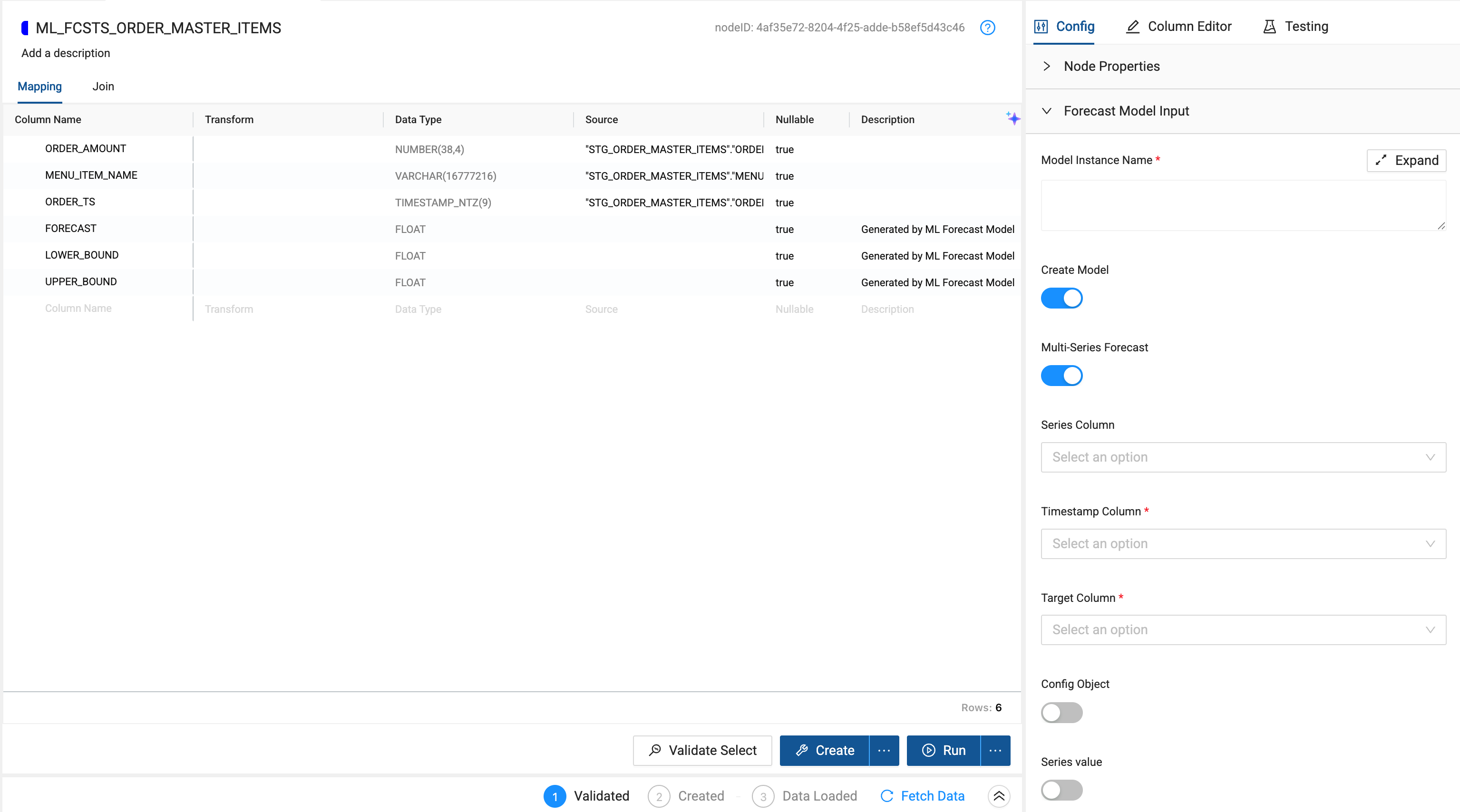
Navigate back to the Browser to see your data pipeline. Select the STG_ORDER_MASTER_ITEMS node that we have been working with and right click on it. Select Add Node -> CortexML -> Forecast.
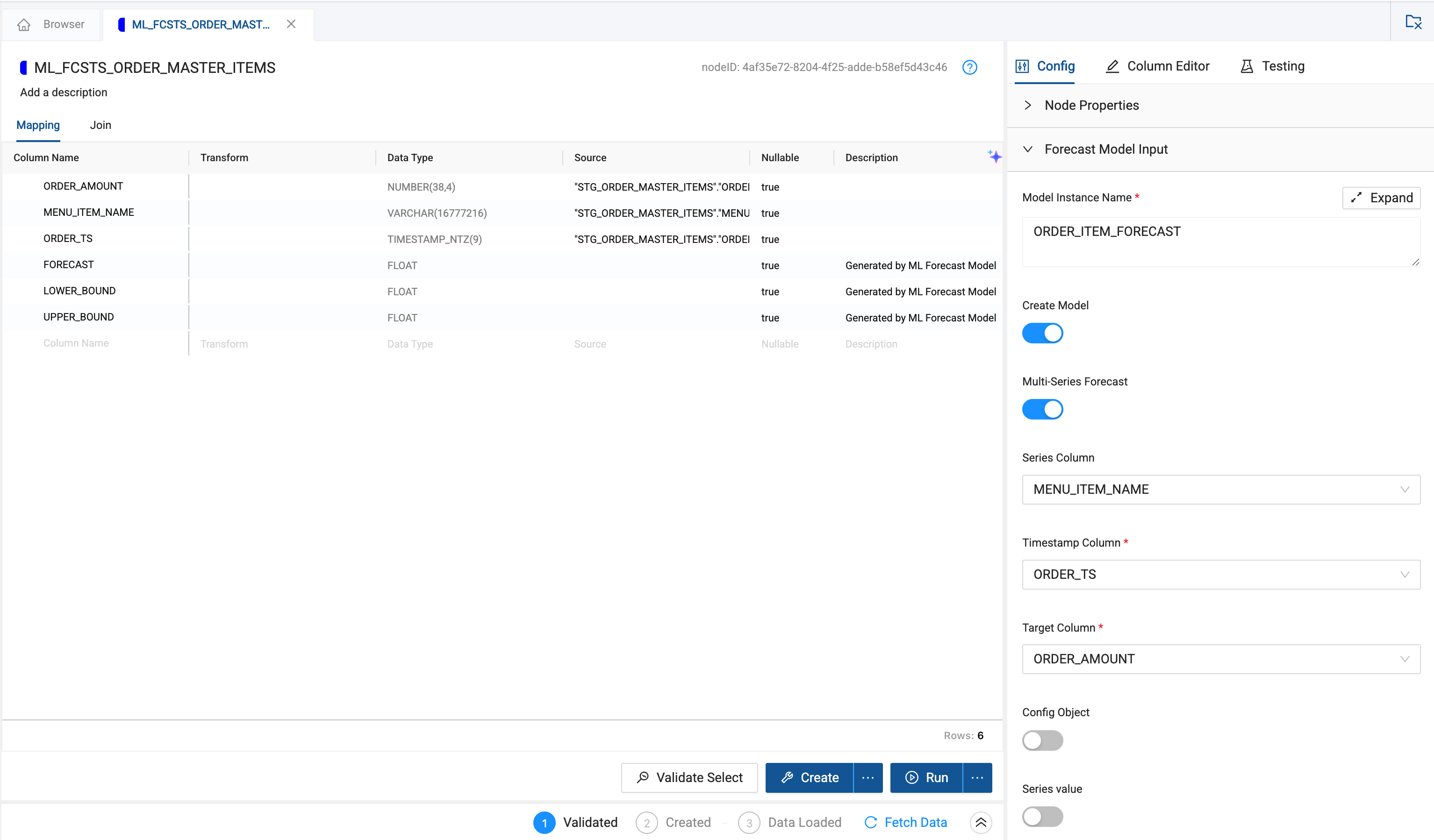
Within the node, there will be three additional columns that have been added, FORECAST, LOWER_BOUND, and UPPER_BOUND. These are generated automatically by the ML Forecast node and will be used to forecast the values of the configured node.

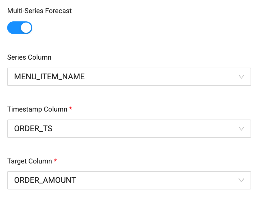
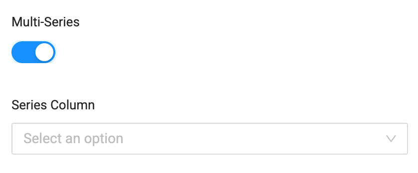
Within the config section, select the Forecast Model Input dropdown. This is where we will configure the node to forecast the values we want to predict. Since there are multiple menu items that we will be predicting order amounts for, we will leave the Multi-Series Forecast toggle to on.
For the Model Instance Name, you can name the model any meaningful name you want, but for the sake of this lab, we will call this model ORDER_ITEM_FORECAST.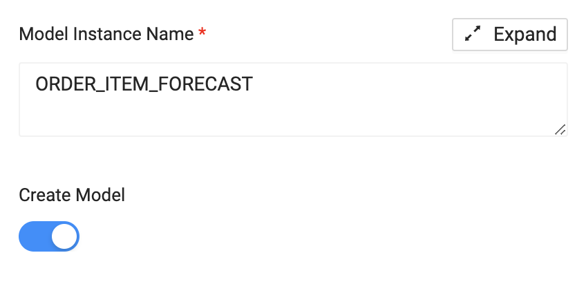
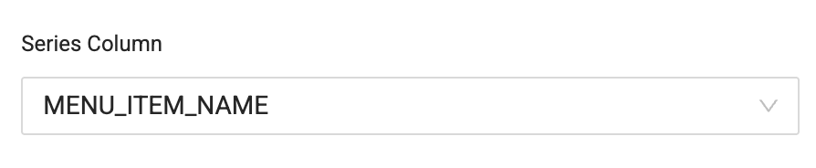
For the Series Column input, we will use the FORECAST_MENU_ITEM_NAME column. This Series Column is the column that is used as the series for predicting values for.
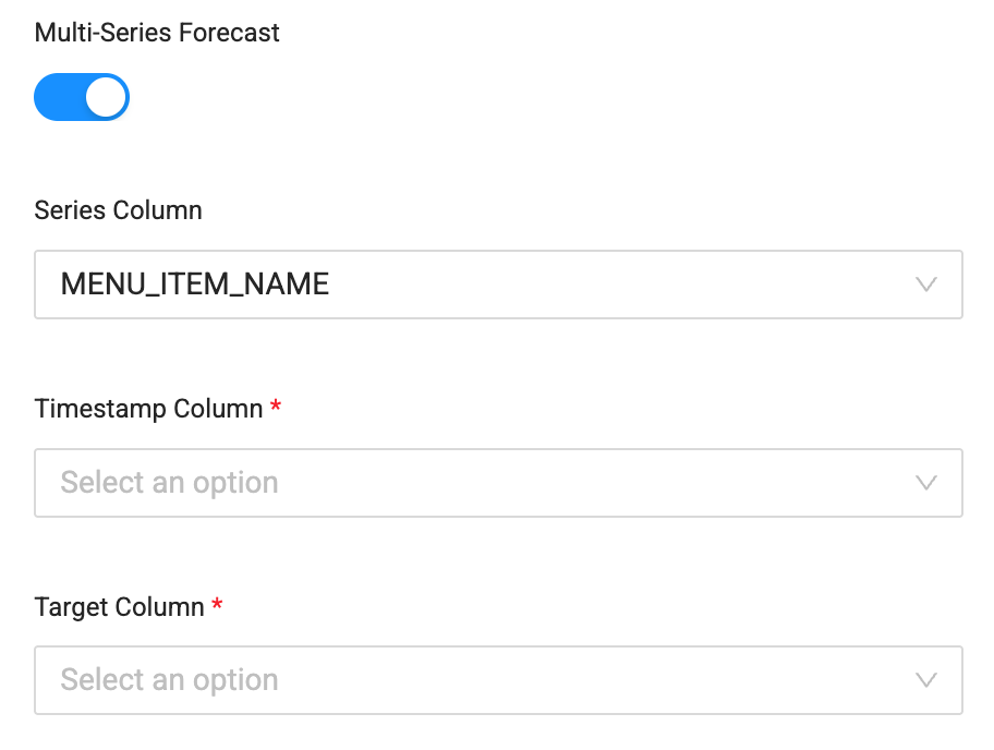
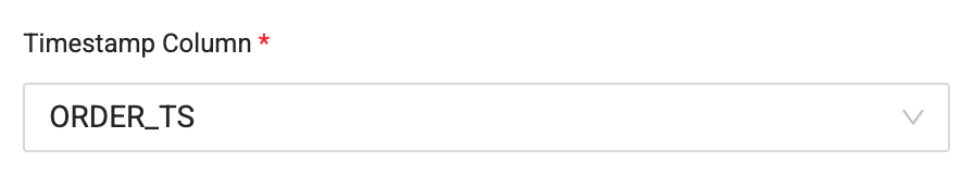
For the Timestamp Column, we will use the FORECAST_ORDER_TS column.
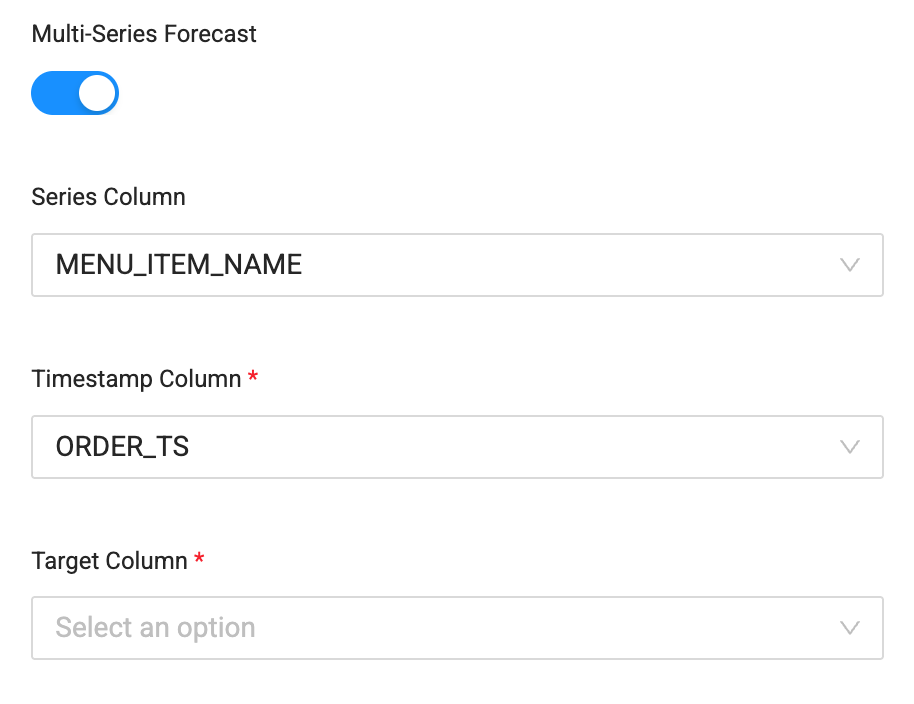
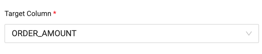
For the Target Column, we will use the FORECAST_ORDER_AMOUNT column. The Target Column is the column that contains the values we want to predict.
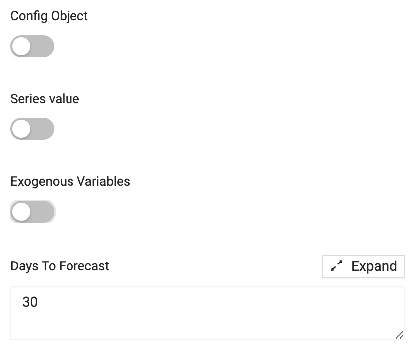
In this node type, the exogenous variables toggle is turned on. Exogenous Variables are additional features or columns that the model can use to help refine and predict the output for the model. Our node doesn’t contain any additional columns that are not being used by the required parameters, so we will toggle this off.

We are presented with a Days to Forecast input that defaults to 30 days. We can update this value to any value of our choosing, but for the sake of this lab guide, will leave the value at 30.
You have now successfully configured the ML Forecast node. Create and Run the node to populate it within Snowflake.

Creating an Anomaly Detection Model

Now that you have created your sales forecast, you can view both your historical and forecasted data to look for anomalies that your forecast may not have taken into account. The final step of this pipeline will be adding the Anomaly Detection node.

Within the ML_FCSTS_ORDER_MASTER_ITEMS node, select the FORECAST_ORDER_TS, FORECAST_ITEM_NAME, and FORECAST columns.
Right click on either of the columns and select Add Node -> View.
We are adding a view so we can filter our data for only forecasted values, without impacting the forecast node we created in the previous step. Rename the view node to V_ORDER_MASTER_ITEMS.
Navigate to the join tab and use a filter for only non null values in the FORECAST column. Effectively, we only want to return values that have a forecasted value, not the entire population from the forecast node. You can either write, or copy the filter below to apply this:
```
WHERE "FORECAST" is not null
```
Rename the FORECAST column to FORECAST_PRICE. Create the view and ensure that there are values in the forecast column.
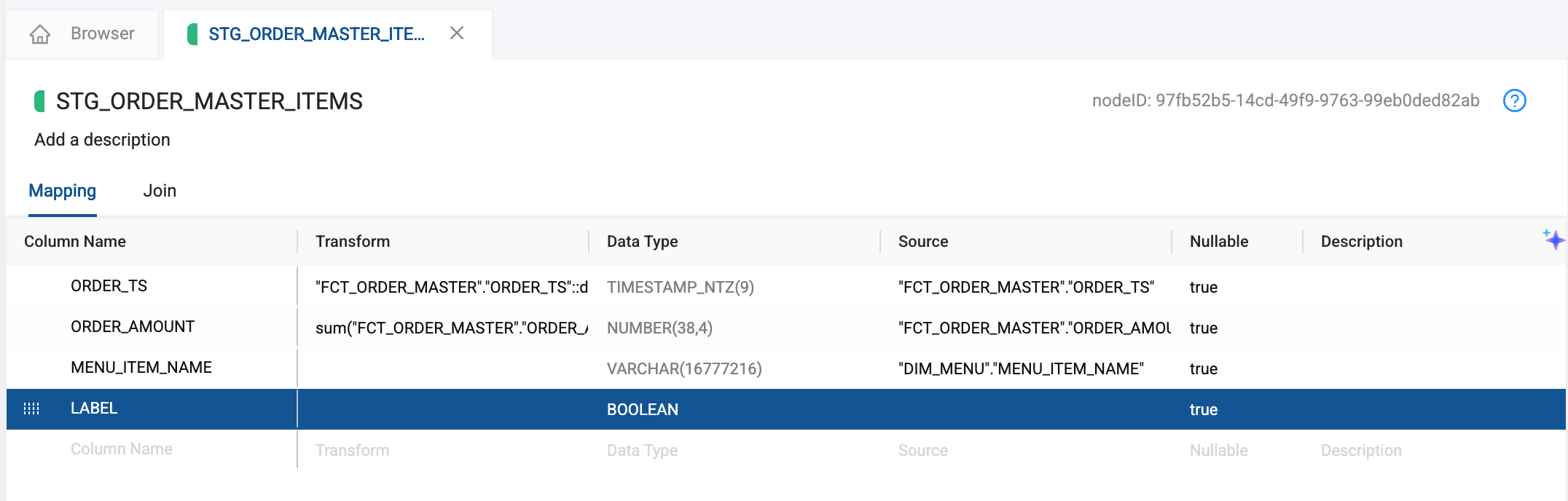
In order to look for anomalies in our forecast data, we need to train our anomaly detection model on historical data. Open the STG_ORDER_MASTER_ITEMS node, which contains all of our historical orders data.
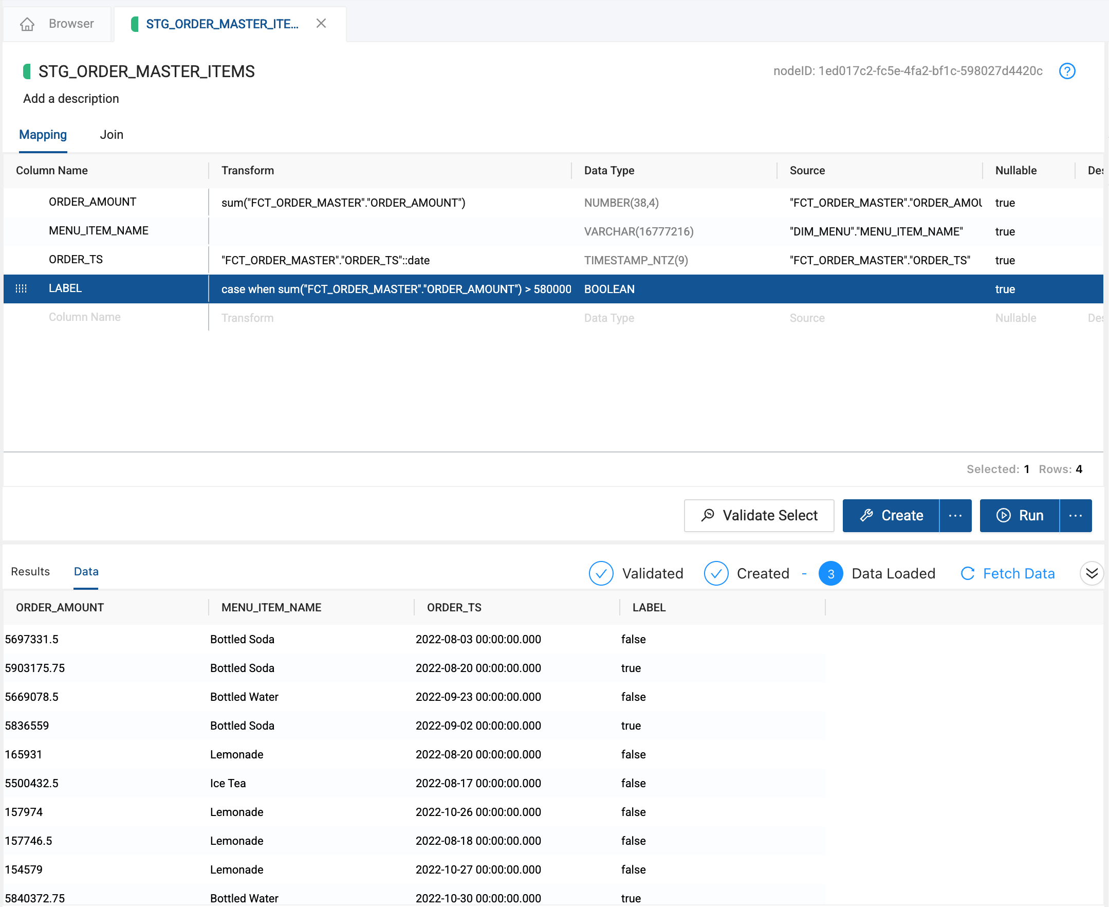
Create a new column called LABEL and add a data type of BOOLEAN. This will be our training set where we tell the anomaly detection model what should be considered an anomaly.
In the transformation field of the LABEL column, add the following transformation:
```
case when FORECAST_ORDER_AMOUNT > 5500000 then TRUE else false END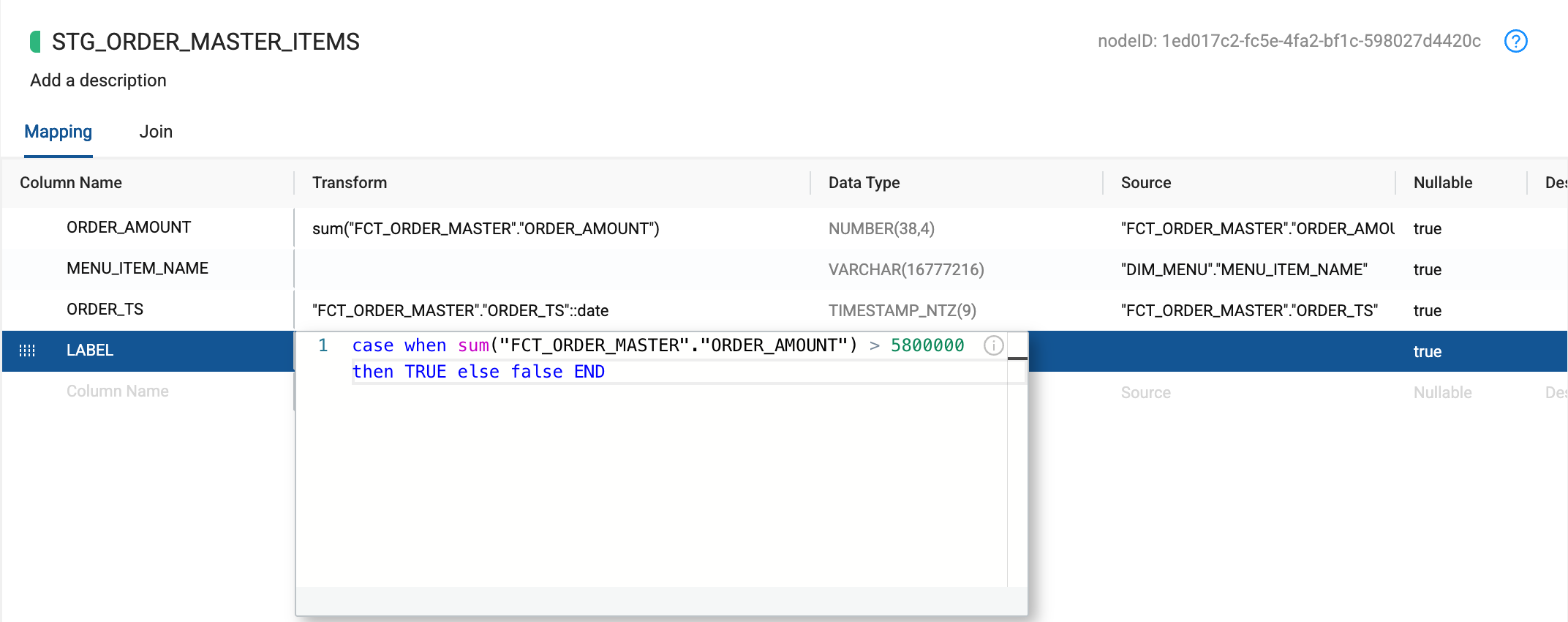
```
Create and Run the node to populate it with the new column and data. Fetch the data to ensure the logic in your transformation is working.
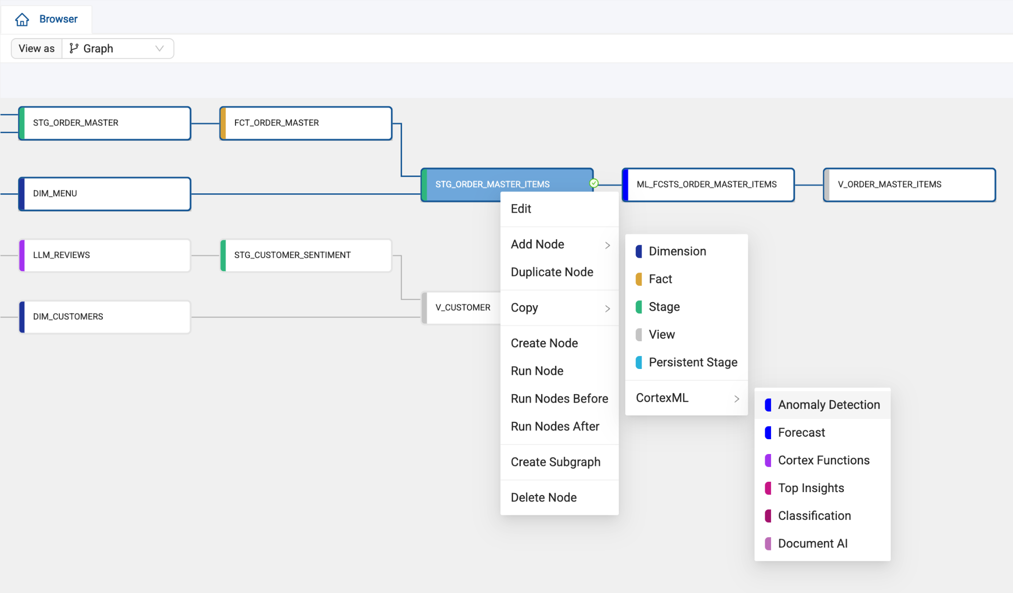
Back in the Browser, right click on the STG_ORDER_MASTER_ITEMS node and select Add Node -> CortexML -> Anomaly Detection.
Open the Anomaly Model Input settings in the configuration on the right side of the screen. We'll need to configure these parameters to build our anomaly detection.
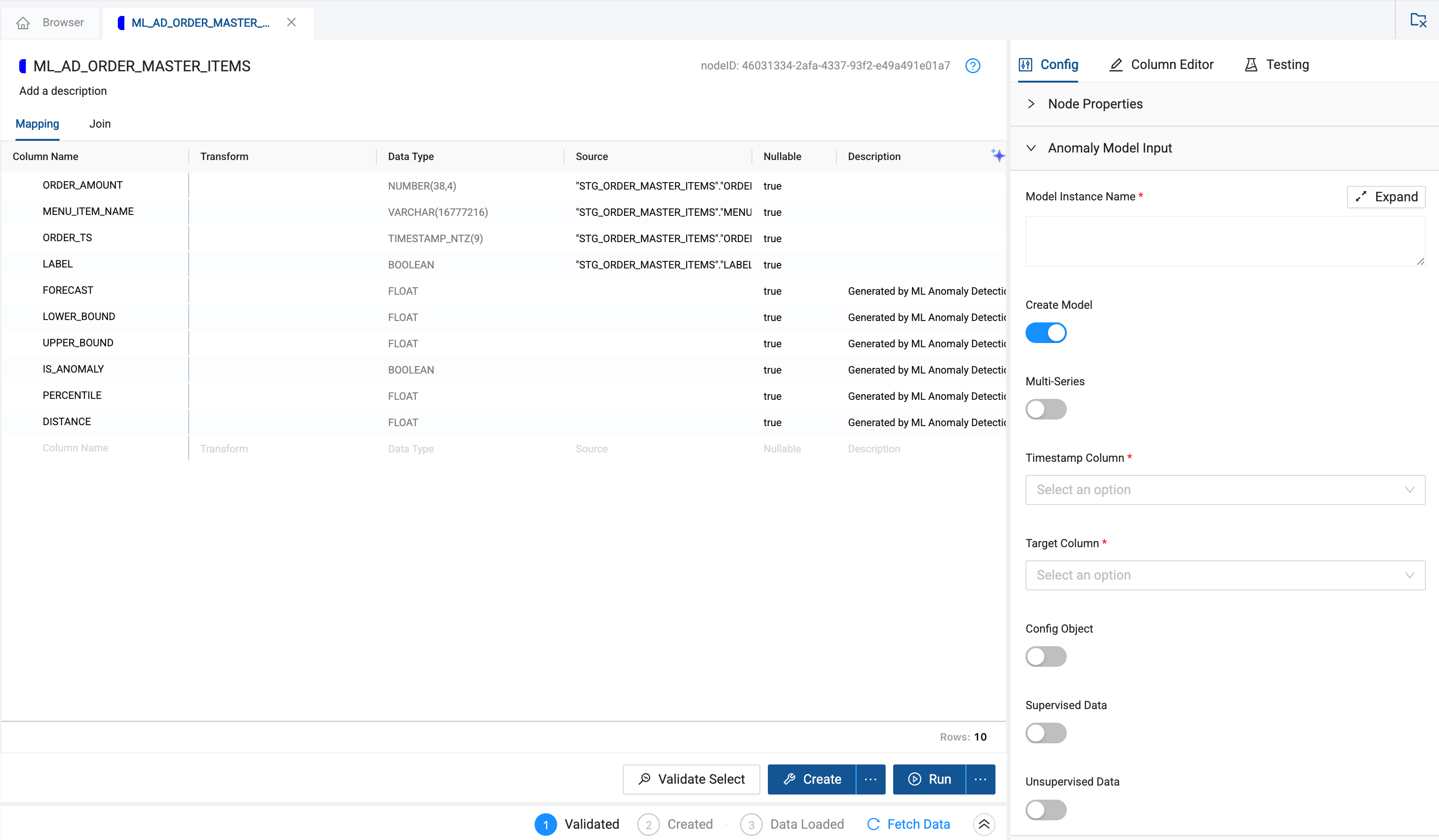
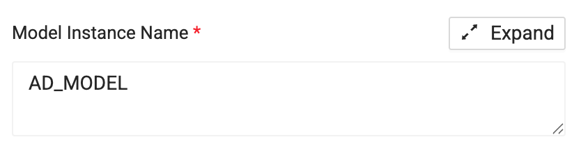
First, give the model instance a name, in this case we'll call this AD_MODEL.
Since we have multiple menu items we are looking at anomaly detection for, toggle the Multi-Series toggle to on.
For the Series Column, select the FORECAST_ITEM_NAME column.
For the Timestamp Column select the FORECAST_ORDER_TS column.
For the Target Column select the FORECAST_PRICE column.
Finally, toggle the Supervised Data toggle to on, becasue we will be training our model on the data we labled in the Stage node we were previously working in.
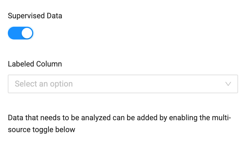
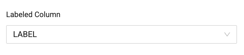
For the Labeled Column, select the LABEL column.
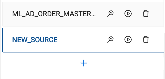
Now we need to add in the dataset that we want to evaluate for anomallies. Select the Multi Source toggle to turn it on so we can bring in our forecast data to evaluate for anomalies.
In the Multi Source pane next to the mapping grid, select the plus + button to add the forecast data to our model.
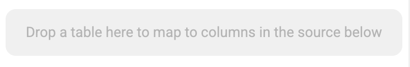
In the node navigation on the left side of your screen, drag and drop the V_ORDER_MASTER_ITEMS node into the table column mapping.
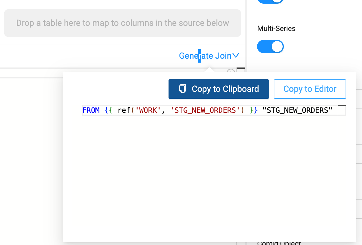
Coalesce will map the existing column to the historical dataset. Navigate to the join tab so you can create the dependency for the new data source. You'll see that the SQL editor is blank.
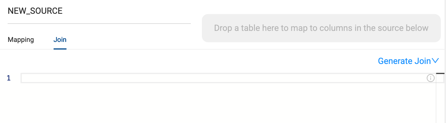
Select the Generate Join dropdown to establish the dependency by selecting Copy to Editor.
Now, Create and Run the node. It may take a minute or two to run depending on your warehouse size.

Conclusion and Next Steps

Congratulations on completing your lab. You've mastered the basics of Coalesce and are now equipped to venture into our more advanced features. Be sure to reference this exercise if you ever need a refresher.

We encourage you to continue working with Coalesce by using it with your own data and use cases and by using some of the more advanced capabilities not covered in this lab.

What we’ve covered

How to navigate the Coalesce interface
Configure storage locations and mappings
How to add data sources to your graph
How to prepare your data for transformations with Stage nodes
How to join tables
How to apply transformations to individual and multiple columns at once
How to configure and understand the ML Forecast node

Continue with your free trial by loading your own sample or production data and exploring more of Coalesce’s capabilities with our documentation and resources. For more technical guides on advanced Coalesce and Snowflake features, check out Snowflake Quickstart guides covering Dynamic Tables and Cortex ML functions.

Additional Coalesce Resources

Reach out to our sales team at coalesce.io or by emailing sales@coalesce.io to learn more.

Overview​

What You’ll Need​

What You’ll Build​

What You’ll Learn​

About Coalesce​

What Can You Do With Coalesce?​

How Is Coalesce Different?​

Core Concepts in Coalesce​

Organization​

Projects​

Workspaces VS Environments​

Lab Use Case​

Before You Start​

Step 1: Create a Snowflake Trial Account​

Step 2: Create a Coalesce Trial Account with Snowflake Partner Connect​

Step 3: Set Up The Dataset​

Step 4: Add the Cortex Package from the Coalesce Marketplace​

Navigating the Coalesce User Interface​

Configure Storage Locations and Mappings​

Adding Data Sources​

Creating Stage Nodes​

Exploring the Node Editor​

Applying Single Column Transformations​

Joining Nodes​

Creating Dimension Nodes​

Creating A Fact Node​

Using Cortex Nodes for Processing Data​

Creating ML Processing Node​

Transforming Data in a Node​

Adding an ML Forecast Node​

Creating an Anomaly Detection Model​

Conclusion and Next Steps​

What we’ve covered​

Additional Coalesce Resources​